MotrixSim
Technical Report
Making physical interaction a scalable, generative learning resource
Contents / 目录
1Understanding MotrixSim
AI is moving from the digital world into the physical one. Vehicles, industrial equipment, construction machinery, and robots are evolving from machines that execute preset programs into intelligent systems that perceive their environment, adapt their decisions, and continuously improve their behavior. Their forms and tasks differ widely, yet they share the same challenge: how to acquire reliable acting capability in a complex, changing real world where trial and error is expensive.
The role of simulation is expanding accordingly. In traditional workflows, simulation answered questions such as “is this structure reliable”, “how does this vehicle respond under this condition”, or “does this control scheme meet requirements” — humans propose a design, and simulation helps them analyze and verify it. Physical AI — intelligent systems that must sense, decide, and act on the physical world — brings a different mode of use: an intelligent system repeatedly tries in a virtual environment, accumulating interaction experience under varying loads, friction, terrain, and disturbances; training perception from synthetic observations; refining behavior through physical feedback; and exploring dangerous, rare, or costly conditions before deployment. Simulation is no longer only the exam hall where a finished intelligent system is tested — it is becoming the training ground where its capabilities are formed. This demands simulation that combines trustworthy physical interaction, efficient computation, and multimodal environmental feedback.
MotrixSim is built around this need as a simulation foundation for physical AI: describing the physical consequences of actions through fine-grained contact, complex geometry, and multibody dynamics; scaling testing and learning through CPU/GPU parallel computation; and connecting environmental observation with behavioral feedback through vision, geometric sensing, and touch. The goal is not merely to get a virtual scene running, but to make physical interaction something that can be repeatedly generated and systematically explored, and then used to train, validate, and optimize intelligent systems.
Underpinning all of this remains the classic balance between accuracy and computational efficiency: finer geometry, more complex contacts, and stricter numerical solving typically mean higher cost, and different industries and tasks weigh this balance differently. Pursuing accuracy alone may limit training and iteration speed, while pursuing throughput alone may lose the physical details that determine task success or failure. What we care about is not merely how many simulation steps can be advanced per second, but how much physically meaningful interaction, valuable to the target task, can be delivered within a limited compute budget — from robotic manipulation to vehicle control, from industrial mechanisms to heavy machinery, lowering the cost of acquiring physical experience so that more expensive, high-risk exploration happens first in the virtual world.
2Physics Simulation
2.1Multibody Dynamics
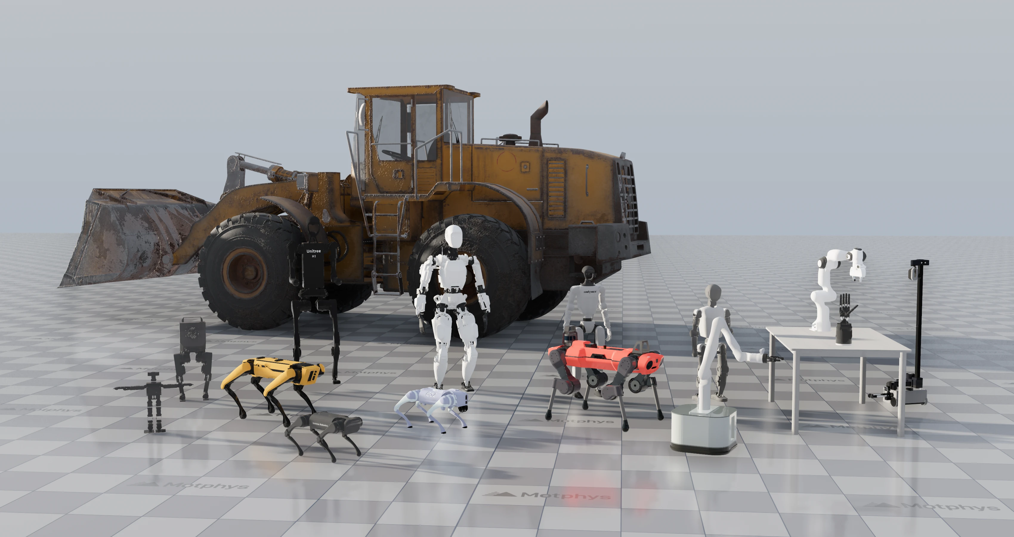
Multibody dynamics describes the overall motion of multiple rigid bodies connected through joints. From humanoid and quadruped robots to robotic arms, dexterous hands, and construction machinery, MotrixSim can model and simulate their whole-body motion. The action of a single joint, a single contact, or a load change can propagate through the joint connections and affect the posture and forces of other parts.
The key to multibody dynamics is not advancing each part separately, but solving the entire joint system as one coupled whole. MotrixSim uses generalized coordinates to describe the motion each joint permits, a mass matrix to represent the inertial coupling between parts and joints, and then maps gravity, actuation, damping, contacts, and external disturbances uniformly into generalized forces acting on the system. The action of one joint, or the force produced by a single contact, therefore propagates to other parts through the dynamic coupling.
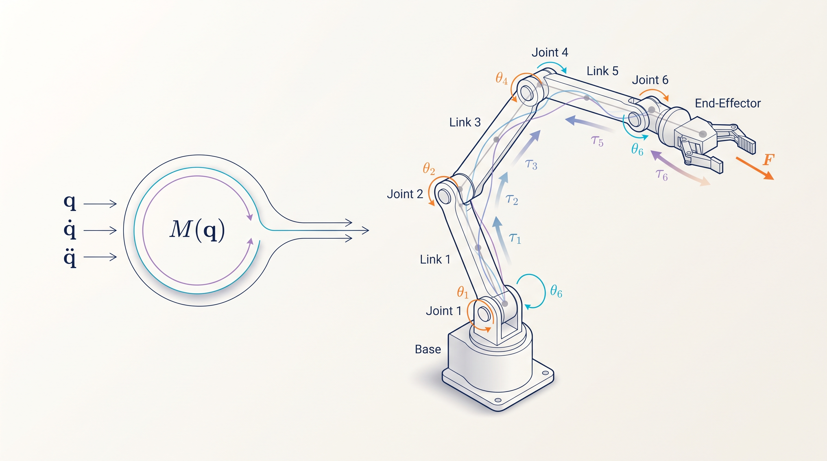
Joint constraints enter the same solving process directly. At each simulation step, the solver simultaneously handles joint connections, joint limits, contact, and friction constraints, computing the generalized impulses or constraint forces needed to satisfy them. As a result, joint motion is not first integrated independently and then pulled back with geometric corrections; instead, the joint-permitted relative motion is maintained within the dynamics solve, and the assembly relationships of closed-loop mechanisms respond jointly to actuation and external forces.
The value of whole-system solving is that local inputs produce global responses consistent with the system structure. Changing the payload at the end of a robotic arm affects not only the end effector but the joint forces along the entire kinematic chain; when a quadruped robot lands, the foot contact forces propagate through the legs to the trunk. Developers can therefore verify, within a single simulation, the interplay between load changes, joint actuation, external disturbances, and environmental contact.
2.2Contact and Grasping
Nearly all multibody systems interact with objects in their environment through contact, and among contact simulations, grasping experiments are particularly critical, as they test a simulator’s stability and physical fidelity under precise, contact-rich conditions. We designed qualitative and quantitative experiments to evaluate how simulators perform on relevant tasks.
Below is a grasping test in which a Franka arm grasps objects of different shapes. Across several simulators, we use identical control trajectories to let the Franka grasp the objects and then compare their robustness to disturbances.
The table below shows each simulator’s configuration and the experiment results.
| Engine and configuration | Ball | Cube | Bottle | |||
|---|---|---|---|---|---|---|
| 2 ms | 10 ms | 2 ms | 10 ms | 2 ms | 10 ms | |
| MotrixSim | ● | ● | ● | ● | ● | ● |
| Isaac Sim | ● | ● | ● | ● | × | × |
| Genesis | × | × | ● | ● | ● | ● |
| MuJoCo Euler | × | × | × | × | × | × |
| MuJoCo Implicit | × | × | × | × | × | × |
| MuJoCo Implicit + no-slip | × | × | × | × | ● | × |
● Pass × Drop. Pass means the run reached 20 s without triggering the drop criterion; it does not imply zero slip. We found that MotrixSim maintains grasp stability across multiple object shapes and step sizes.
After the qualitative tests above, we further evaluated quantitatively whether each simulator’s behavior near the friction-cone threshold stays consistent with theory. For a cube held at rest by a two-finger grip, if N is the sum of the normal gripping forces on both sides, the Coulomb friction model gives the support condition μN ≥ mg, corresponding to the critical friction coefficient μcrit = mg/N. Starting from a stable grasp, the test adjusts the friction coefficient around this critical value and continues simulating for 5 seconds to observe the slip distance.
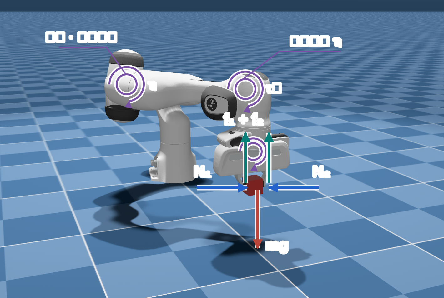
The table below shows three representative test points near the critical friction. MotrixSim slips at 0.98 times the critical value and holds at and above the critical value; both MuJoCo configurations slip at the critical value, and FastImplicit reduces the slip distance to 11.3 mm at 1.10 times the critical value, but still fails the original test criterion as slip.
| μ / μcrit | Theoretical expectation | MotrixSim | MuJoCo Euler | MuJoCo FastImplicit |
|---|---|---|---|---|
| 0.98 | Slips | 150.0 mm✓ Consistent | 153.2 mm✓ Consistent | 150.9 mm✓ Consistent |
| 1.00 | Holds | 0.0 mm✓ Consistent | 151.2 mm× Deviates | 151.7 mm× Deviates |
| 1.10 | Holds | 0.0 mm✓ Consistent | 150.5 mm× Deviates | 11.3 mm× Deviates |
✓ Consistent with theory× Deviates from theory The criterion is "slips below the critical friction coefficient, holds at or above it."
These results show that, under the tested gripping conditions, MotrixSim not only maintains the grasp but also exhibits hold-and-slip behavior near the critical friction consistent with theoretical expectations. For control and policy learning that rely on contact feedback, this is more meaningful than demonstrating a single successful grasp: simulation must provide trustworthy physical boundaries, not merely keep the object from falling.
2.3Rolling Friction and Rotational Dynamics
Beyond sliding friction, rolling friction also plays an important role in simulating wheeled structures. It affects not only rolling decay but also the trajectories of rotating bodies. Below, two physical scenarios — a ball rolling down an incline and a backspin ball — are used to evaluate the accuracy of physics engines in handling rolling friction.
Rolling resistance experiment
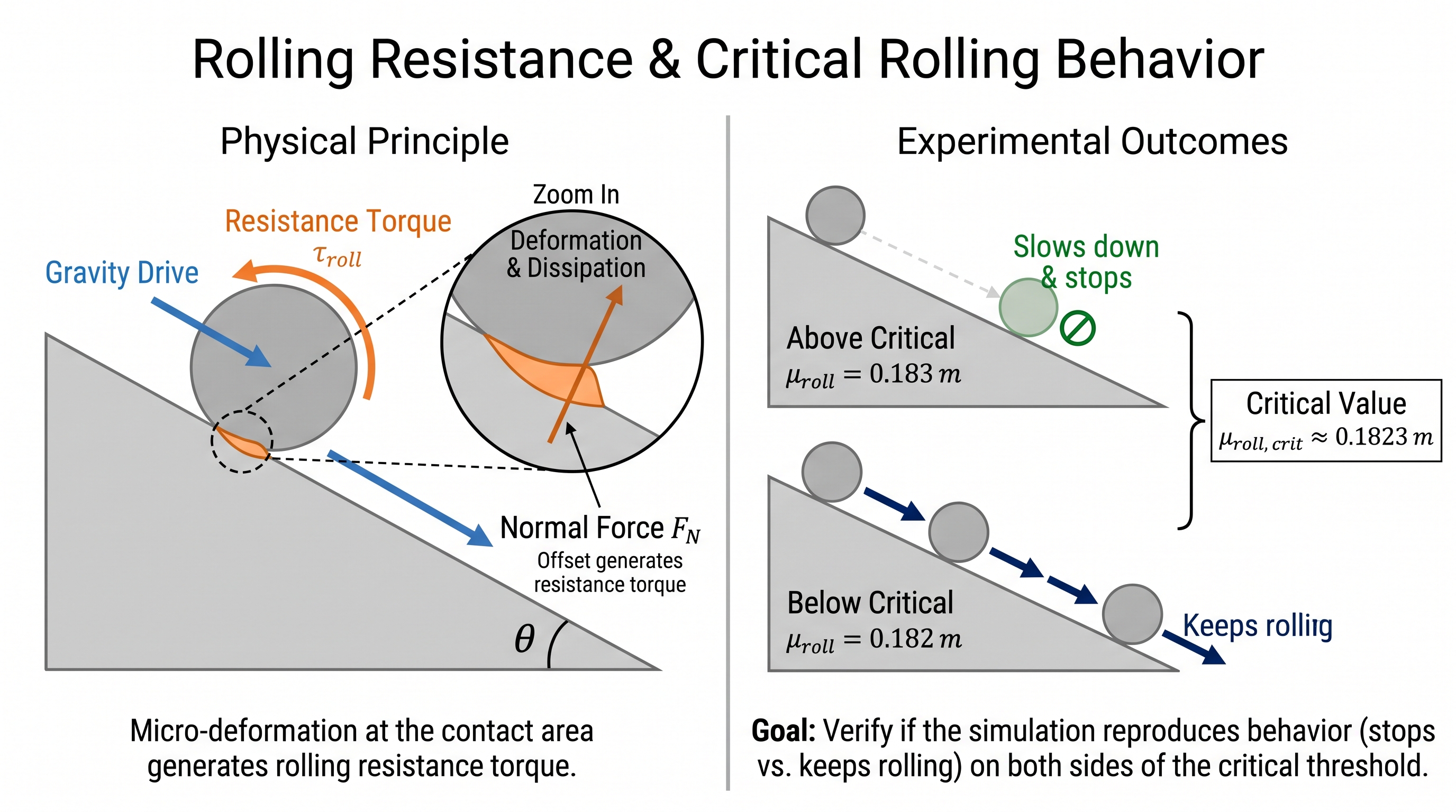
The rolling resistance torque opposes rolling and dissipates energy during it. In this scenario, computed from the ball radius and the incline angle, the critical rolling resistance coefficient is . Above this coefficient the ball should gradually slow down and stop on the incline; below it the ball should keep rolling down the slope. Below we take , slightly above the critical value, and , slightly below it, and compare the two engines.
MotrixSim clearly shows the difference in motion on either side of the critical value: with the coefficient at 0.183, the ball decelerates and comes to rest on the incline; when the coefficient drops to 0.182, the ball keeps rolling down. MuJoCo fails to stop on the incline under both settings — the ball rolls all the way down and finally stops on the flat ground at the bottom.
Additionally, during testing we found that MuJoCo exhibits high-frequency contact-state switching and violent normal-force oscillation in this experiment, reflecting the instability of its numerical solution in this scenario. Within a mere ~20 milliseconds, the ball touches the ground, leaves it, and touches down again; the normal force drops from about 670 N to zero and then rises back to about 672 N. The repeated liftoffs keep interrupting the rolling resistance torque provided by contact, so the ball bounces its way down the slope and fails to come to rest even when the rolling resistance coefficient exceeds the critical value. In contrast, MotrixSim stably reproduces coming to rest on the incline above the critical value, and continuous rolling below it.
Backspin ball experiment
A backspin ball is like a “draw shot” in billiards: the ball moves forward while carrying a strong reverse spin, then decelerates and reverses under friction.
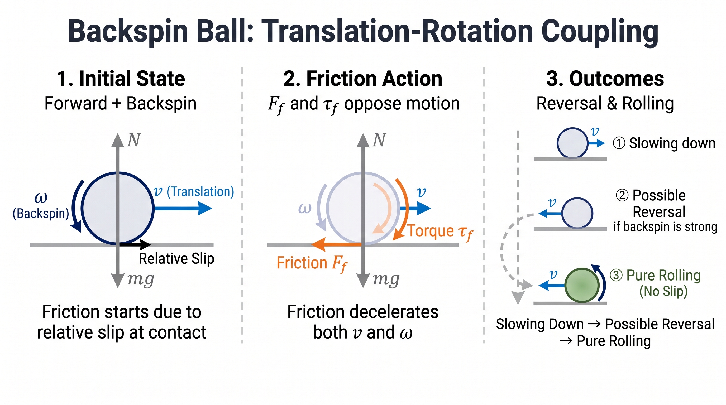
In this scenario’s ideal hard-contact model, the ball starts resting on the horizontal ground with no vertical impact or elastic energy storage. Friction acts along the ground, changing the ball’s horizontal velocity and spin rate; the normal force balances gravity, the net vertical force is zero, and the ball should therefore remain in contact with the ground.
2.4Closed-Loop Mechanisms and Constraints
Some mechanical systems’ motion is not determined by a single joint chain, but jointly constrained by multiple closed loops. In such mechanisms, one actuated input propagates through linkages to multiple branches; every connection point must maintain the correct positional relationship, and a local error can travel through the mechanism to the other side. MotrixSim solves closed-loop constraints together with the multibody dynamics, so the mechanism maintains its assembly relationships during motion.
The Strandbeest illustrates this problem vividly. The model contains 12 legs, 92 linkages, and 36 closed kinematic loops, with all legs driven by the same crank. The simulation does not play back each leg’s trajectory one by one; instead, it computes the motion response of the entire mechanism from the crank input, the linkage masses, and the closed-loop constraints. Consequently, changing the drive speed or the initial posture changes the phase and footfall motion of the whole set of legs accordingly.
This modeling approach also applies to linkage mechanisms, folding mechanisms, and robots with internal closed loops. Developers can combine joint actuation, contact, and closed-loop constraints in the same scene, and observe how mechanism motion, ground contact, and external disturbances interact.
2.5Fine-Grained SDF Collision
In tasks that rely on precise geometric collision — dexterous grasping, gear meshing, precision assembly — local geometry such as grooves, gear teeth, and curvature changes cannot be accurately represented by simple spheres, boxes, or a single convex hull. Once these details are filled in or covered over, contact positions and the space of feasible motion change accordingly.
MotrixSim supports signed distance fields (SDFs), which represent complex curved surfaces and non-convex structures via the signed distance from a spatial position to the surface, preserving the object’s key geometric features. This capability supports multi-point contact between moving objects and static environments, as well as between complex SDF shapes, so that local contours can participate in supporting and constraining the object’s motion.
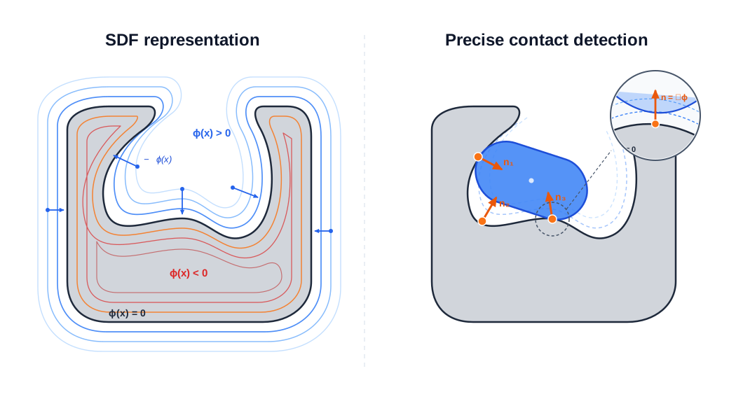
The following three simulation scenarios from MotrixSim demonstrate this capability:
2.6Vehicle Dynamics Simulation
MotrixSim can perform vehicle dynamics simulation and provides all the capabilities needed to build a credible virtual vehicle: suspension and tire modeling elements, a calibration workflow using measured data, scenario and operating-condition demonstrations, real-time execution, and large-scale parallel sampling. This section presents these capabilities through component configuration examples and full-vehicle driving demonstrations: the elastic-element figures use synthetic example data, the tire fitting figures use the publicly available KIT TYDEX bench-test data, and the full-vehicle videos use an independently calibrated model to showcase vehicle dynamics behavior.
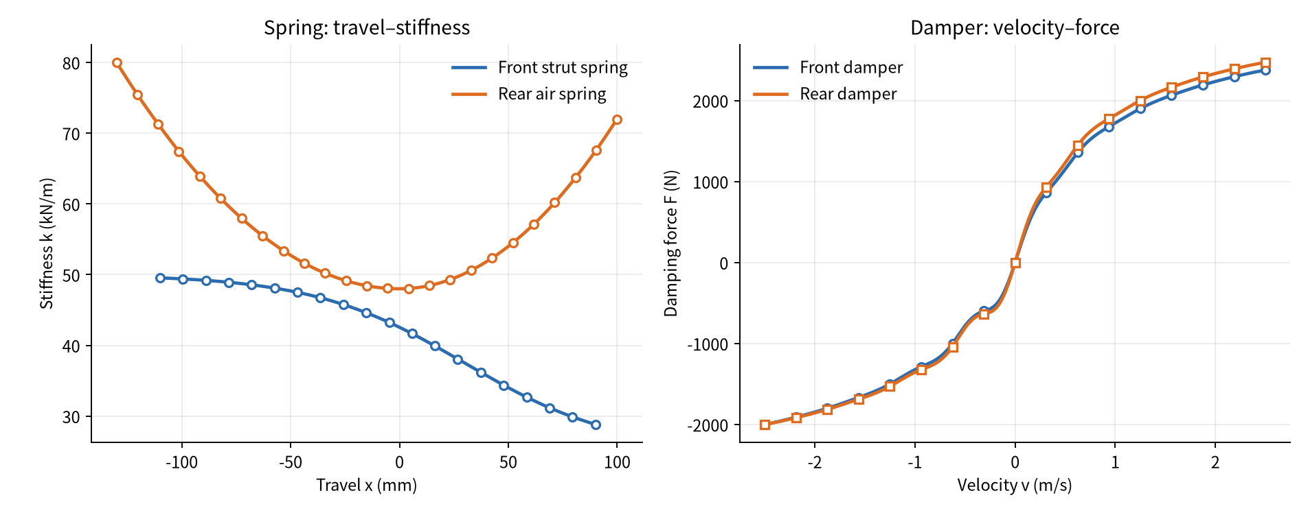
MotrixSim supports nonlinear suspension modeling and organizes reusable vehicle assets through XML configuration. Spring stiffness can vary with travel, damping can be described with a velocity–damping-coefficient table or a velocity–force table, and the compression and rebound sides can be configured separately, making it possible to express progressive stiffness, nonlinear damping, and similar characteristics. Damping levels can also be switched at runtime for semi-active suspension control.
Suspension elements and their characteristic data are configured together with the XML model: when adjusting spring or damper characteristics, you only need to replace the corresponding parameters and data tables, and the vehicle assets and simulation pipeline can be reused. The figure below shows nonlinear spring and damping characteristics using synthetic example data.
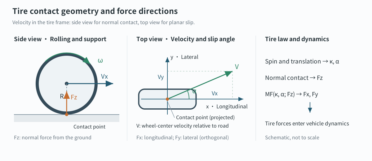
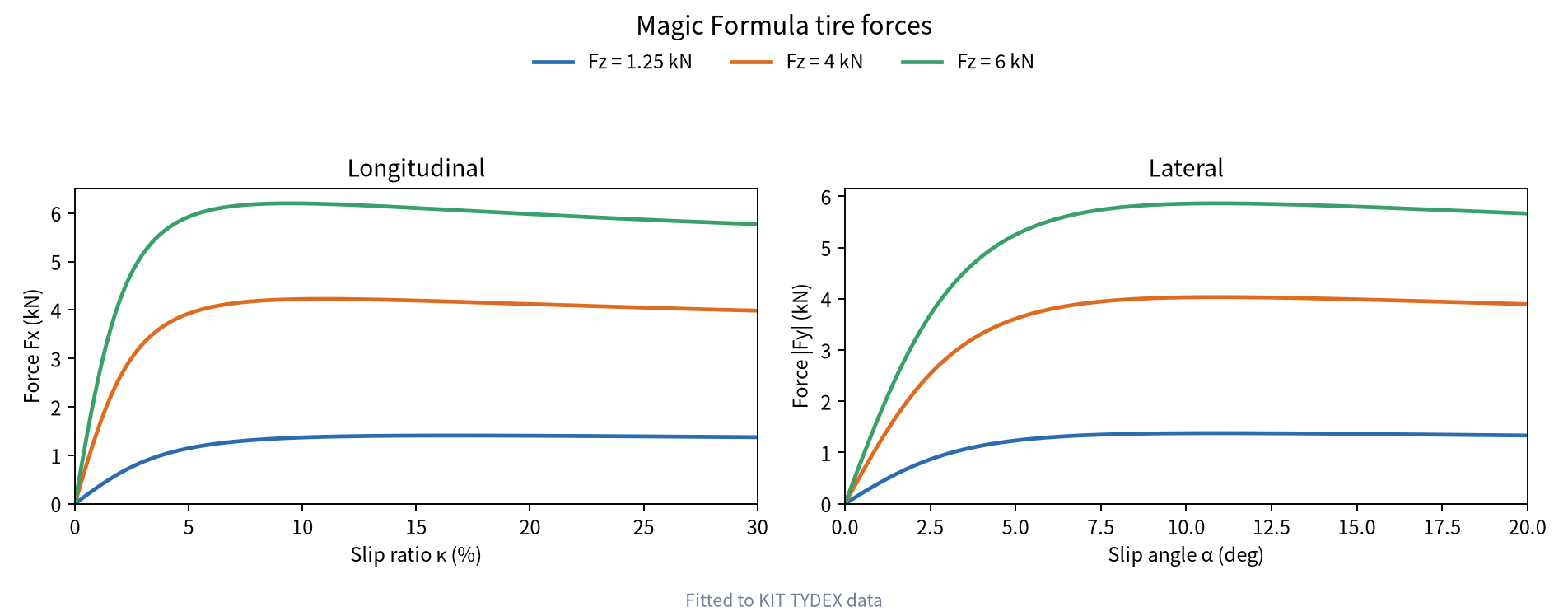
MotrixSim places the Magic Formula inside the contact constraint chain rather than applying it as a separate external force each frame. Collision detection first establishes normal and tangential contact constraints from the geometric relationship between the tire and the road surface, and a custom contact-patch generation method describes the actual tire–road contact area.
The model then computes slip ratio and slip angle from the normal load and local velocity at the contact point, and uses the MF constitutive law to obtain the target longitudinal and lateral force responses. The solver places these responses, the normal support, friction limits, and the full-vehicle mass matrix into a single constraint system, solving for the contact impulses and their reaction forces on the wheels and the body; once body attitude and per-wheel loads are updated, computation continues at the next time step. This unified solve means tire forces are transmitted to the body realistically through the suspension, while load transfer in turn changes tire grip. Acceleration, braking, steering, and road unevenness therefore combine naturally within a single model, without patching in external force rules.
The tire model is inexpensive — each tire occupies only three solver constraints — and is naturally suited to large-scale parallel simulation. The fitting workflow was validated on the public KIT TYDEX dataset (32 files, 1015 operating points), with a median peak-force coefficient error within 3%[1]; the vertical contact stiffness can be back-calibrated against bench tests to a target value. Formulas and symbol definitions are in the appendix.
The scenario demonstrations cover jump ramps, consecutive speed bumps, slalom steering, and emergency lane changes. The ramp-crossing sequence shows the suspension response as the vehicle pitches nose-up on the way up and nose-down on the way down; the consecutive speed bumps compare wheel hop and body vibration at different speeds; the slalom and emergency lane changes show body roll, lateral oscillation, and trajectory tracking during fast steering.
In terms of performance, full-vehicle simulation runs in real time and scales to large-scale parallel sampling. The tested vehicle (103 velocity degrees of freedom) cruises at 60 km/h for 20 s with a 5 ms time step, taking 0.27 ms/step of pure physics time on a single core — about 18.5× real time†; the Newton solver averages 1.01 iterations and never hits the iteration cap in 4000 steps. Scaled up to asynchronous parallel sampling, 1024 environments sustain 17,716 steps/s† — this is sampling throughput and does not imply proportional speedup for higher-level applications. Test conditions are in the appendix.
| Condition | Result |
|---|---|
| Single-environment cruise (103 DOF, 5 ms) | 0.27 ms/step, about 18.5× real time |
| Parallel sampling, 1024 environments | 17,716 steps/s |
2.7Soft-Body Simulation
MotrixSim supports MPM soft body simulation. MPM represents material state with particles and, at each time step, transfers momentum and updates deformation through Particle-to-Grid, grid update, and Grid-to-Particle. It is well suited to describing the compression, rebound, and large deformation of soft bodies under load.
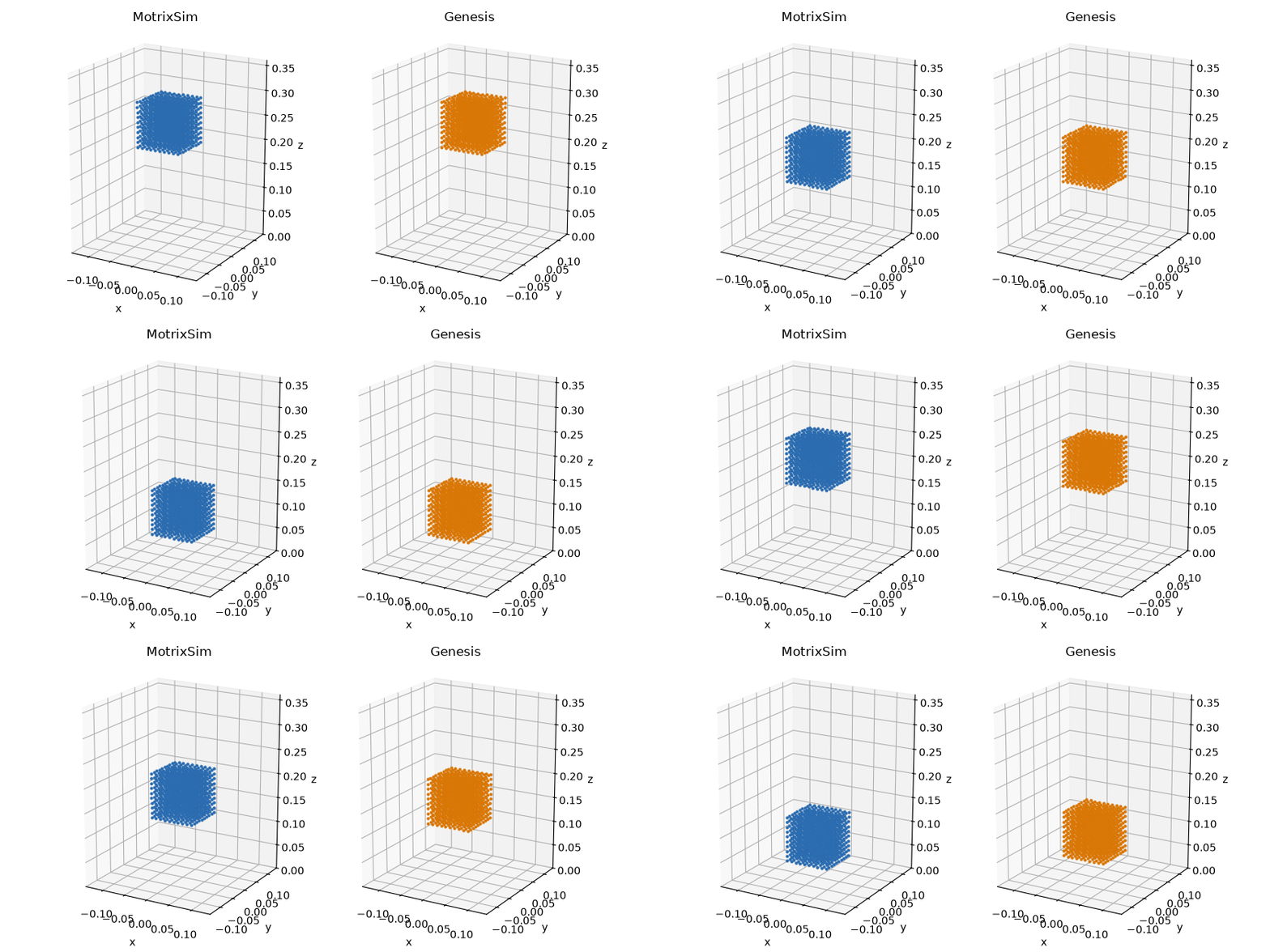
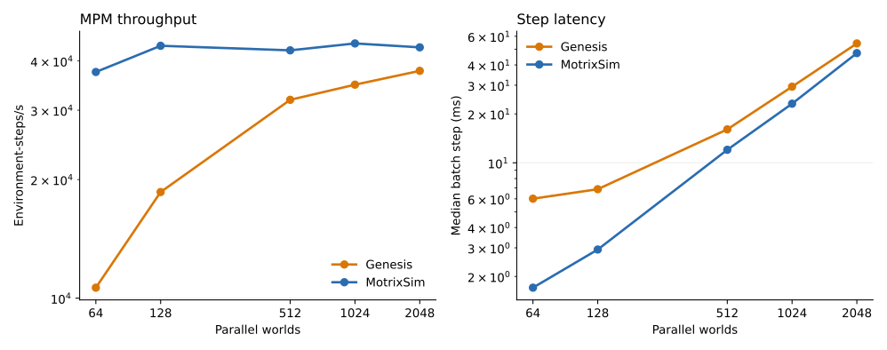
To evaluate the batch performance of soft body simulation, MotrixSim and Genesis use the same Fixed-Corotated soft-cube drop configuration, including the particle array, grid spacing, material parameters, gravity, time step, and ground friction.
| Worlds | MotrixSim step | MotrixSim throughput | Genesis step | Genesis throughput |
|---|---|---|---|---|
| 64 | 1.706 ms | 37,507 env-steps/s | 6.018 ms | 10,634 env-steps/s |
| 128 | 2.928 ms | 43,711 env-steps/s | 6.883 ms | 18,596 env-steps/s |
| 512 | 12.029 ms | 42,565 env-steps/s | 16.061 ms | 31,878 env-steps/s |
| 1024 | 23.107 ms | 44,316 env-steps/s | 29.402 ms | 34,828 env-steps/s |
| 2048 | 47.284 ms | 43,312 env-steps/s | 54.241 ms | 37,758 env-steps/s |
On top of this, MotrixSim further supports rigid–soft coupling simulation. The accuracy of rigid–soft coupled simulation is essential for robotic manipulation tasks involving soft bodies. The following video compares a robotic-arm sponge-grasping task executed in MotrixSim and on a real robot.
2.8Large-Scale Parallel Simulation
Applying simulation to robot reinforcement learning requires massively parallel simulation throughput as an essential capability. Reinforcement learning relies on large-scale interaction sampling from simulated environments to supply gradient data for policy optimization.
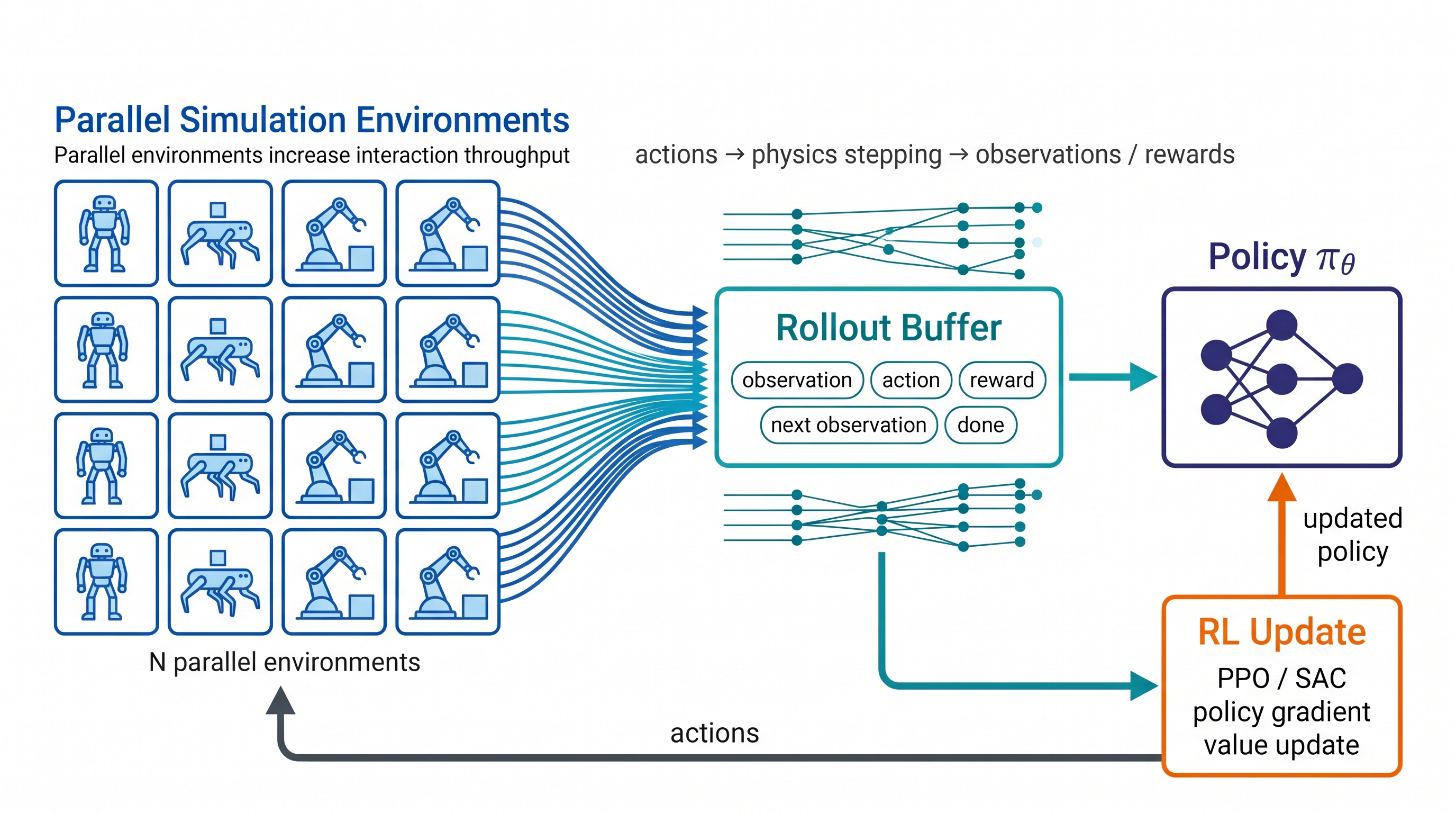
MotrixSim supports both CPU and GPU simulation, and can efficiently advance massively parallel environment simulation on both device types. Below are MotrixSim’s throughput results with 4096 parallel environments; tested devices include a consumer CPU (AMD 9950x), a server CPU (AMD EPYC 9j14), and a high-performance GPU (RTX 5090).
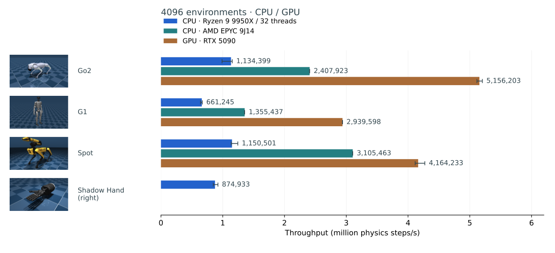
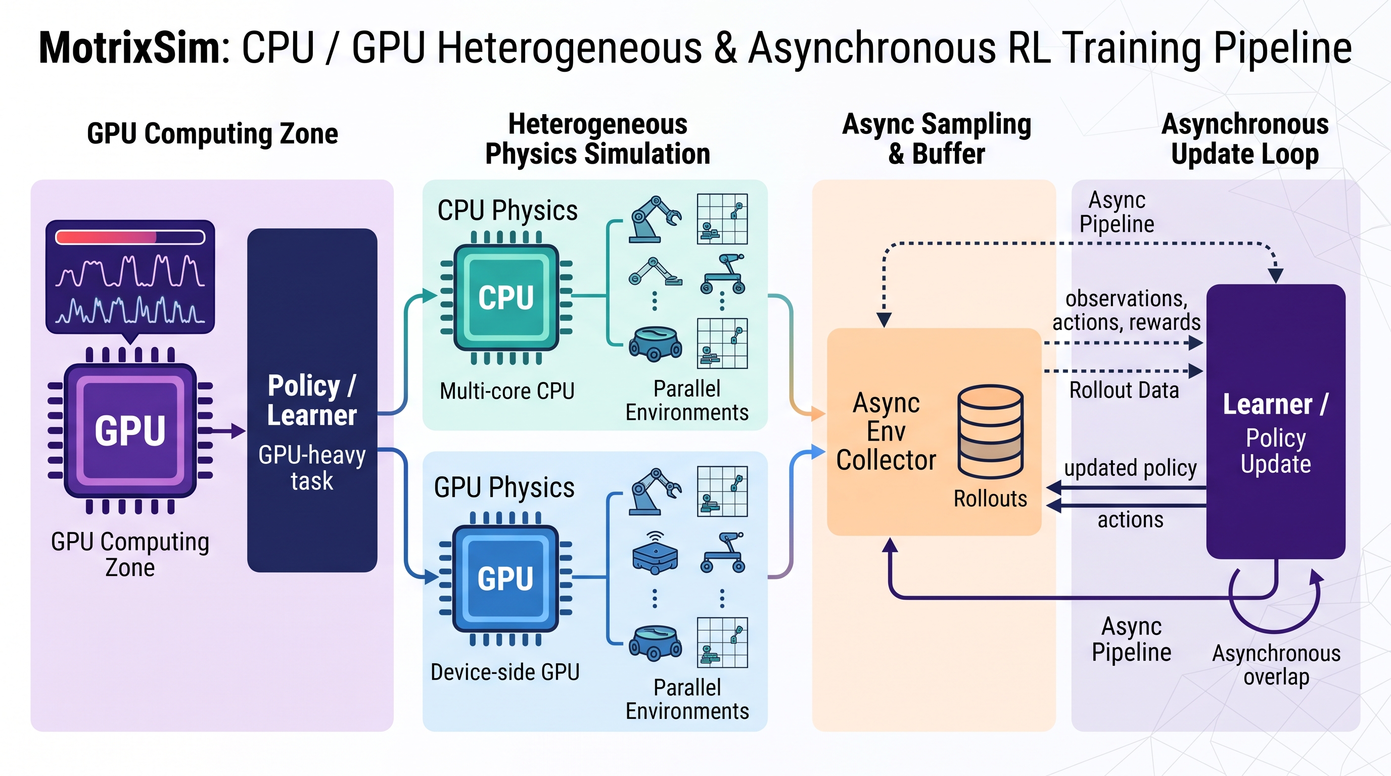
In our tests, we found that through efficient parallel scheduling and batched computation, MotrixSim fully exploits the compute of multi-core CPUs and high-performance GPUs, delivering CPU physics simulation throughput on the same order of magnitude as GPUs (millions of physics steps per second). This efficient use of heterogeneous devices lets us choose the optimal simulation execution path for each hardware configuration, achieving higher efficiency in the end-to-end training loop.
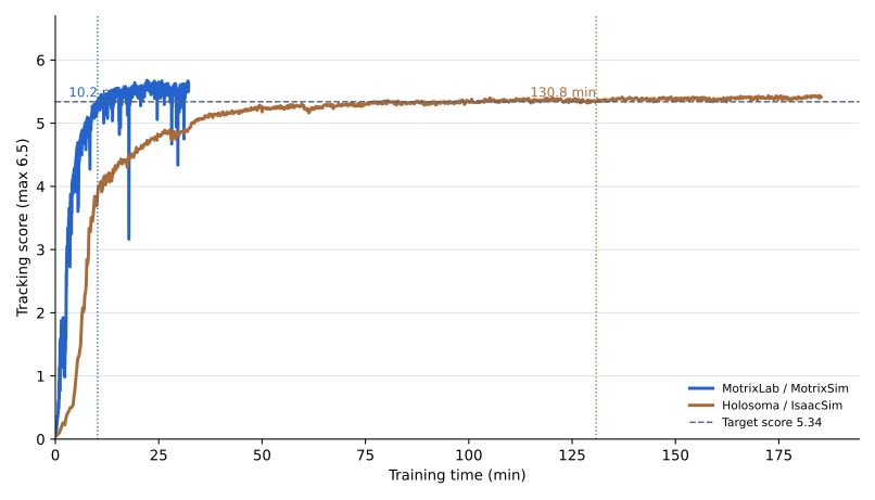
The value of parallel throughput and heterogeneous-device simulation ultimately shows up in training-loop completion time. For the G1 whole-body tracking task, we ran a controlled comparison with the same task environment configuration (including obs and reward), the same RL algorithm (fastsac), and the same hyperparameters. MotrixLab (MotrixSim) reaches the current tracking score in about 10.2 minutes of end-to-end time, while the Holosoma (IsaacSim) reference result is 130.8 minutes — a gap of about 12.8×. These results connect low-level batched physics throughput to real robot-learning workflows: advancing environments faster means the policy collects more interactions in the same amount of time and finishes training earlier.
3Rendering
Physics simulation determines how machines move and interact; rendering turns those states into observable, learnable visual information. For physical-AI tasks, rendering must not only reproduce the appearance of the environment but also stay consistent with the physical scene and efficiently organize many parallel environments into the observations required for policy training. This section first presents hybrid rendering that combines real-world appearance with controllable physical models, then covers image generation and observation output for batched environments.
3.1PBR Rendering
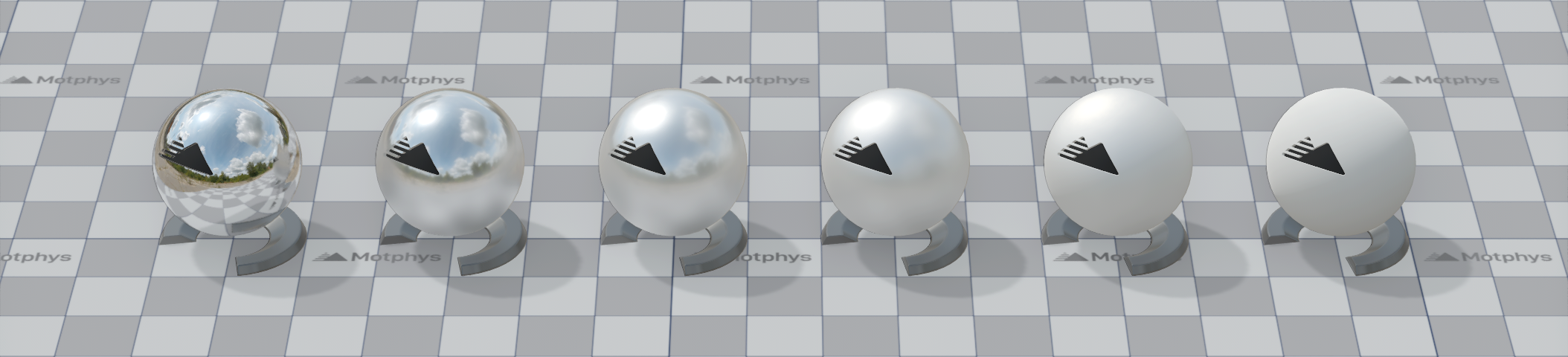
PBR (Physically Based Rendering) describes how surfaces respond to lighting through a set of material parameters with clear physical meanings. MotrixSim combines materials, lights, and environment lighting so that robots and interactive objects not only have color, but also exhibit reflections, highlights, roughness, and metallic appearance consistent with their material properties. For vision-based policies and simulation showcases, this provides a unified appearance foundation for subsequent real-scene fusion.
Material Parameters Determine Surface Appearance
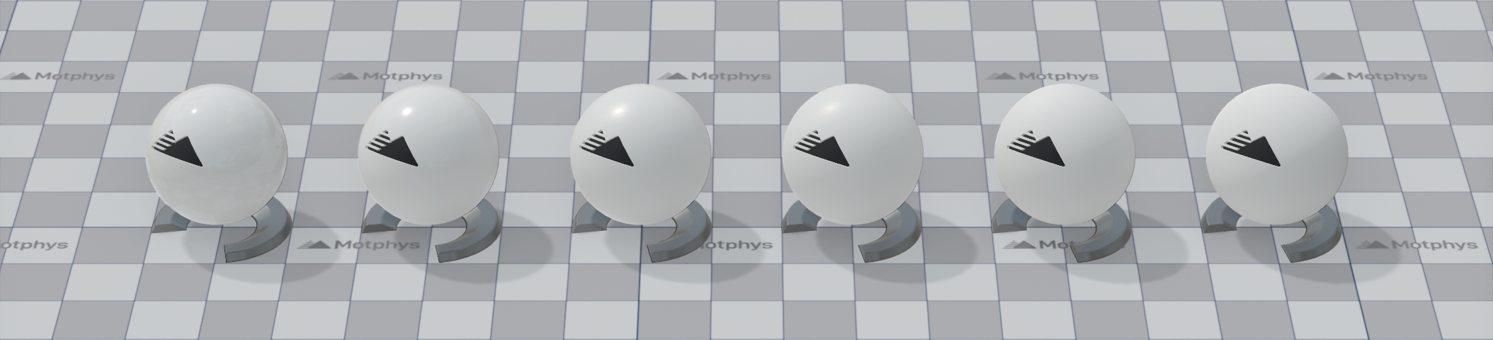
PBR materials are primarily controlled by reflectance, roughness, and metallic. Reflectance determines the reflection strength of non-metallic surfaces; roughness determines how concentrated or diffuse the highlights are; metallic distinguishes the lighting response of metals from non-metals. The parameters have clear meanings and can be configured directly, so the same set of models can express different surfaces such as plastic, rubber, and coated metal by adjusting material parameters.
Screen Space Global Illumination
Screen Space Global Illumination (SSGI) adds indirect lighting to the scene, enhancing the three-dimensionality and spatial depth of objects. MotrixSim approximates the illumination from light bouncing off surfaces within screen space, combined with denoising and spatiotemporal reuse filtering to reduce sampling noise. Occlusion relationships between objects and color bleeding between surfaces become more distinct, allowing materials to blend more naturally with the surrounding environment visually.
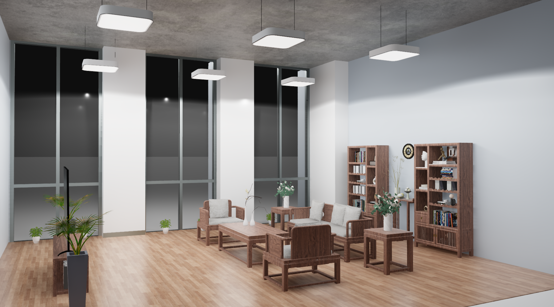
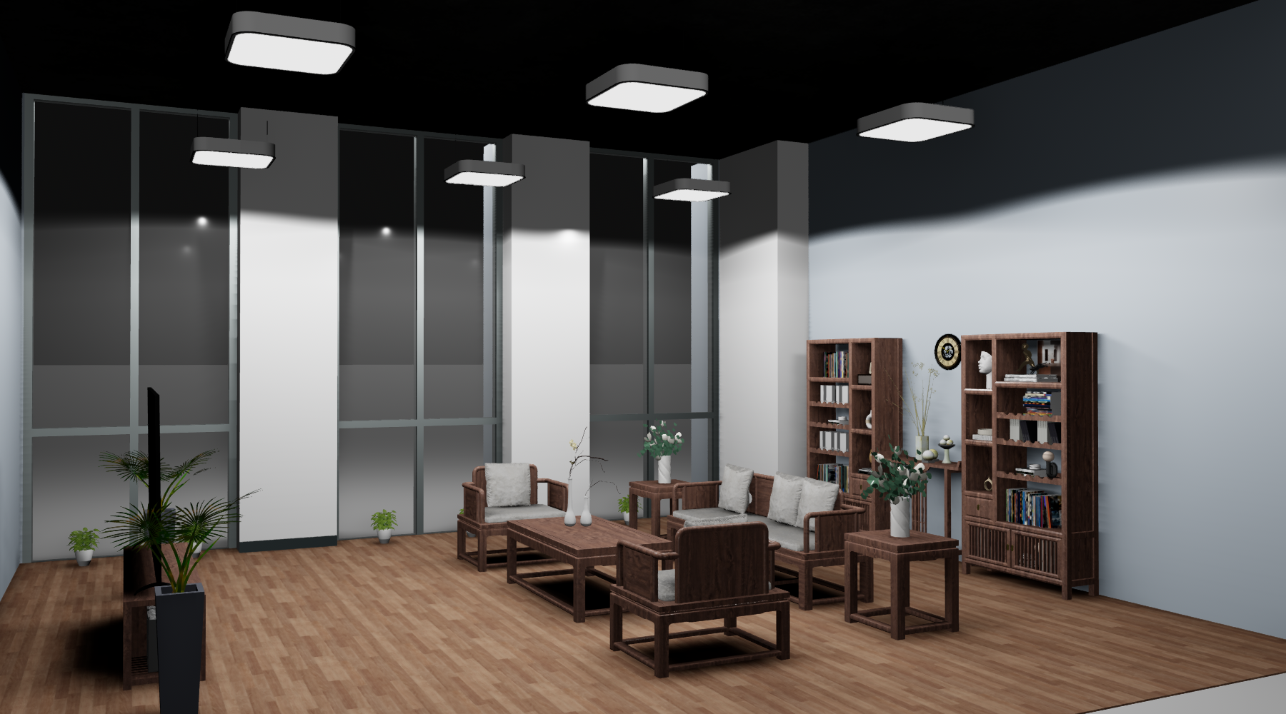
Materials and lighting together determine the appearance of simulated objects. The next section describes how to combine 3DGS scanned scenes so that these objects blend into the visual background of real environments.
3.23DGS Hybrid Rendering
Bring the appearance of real scenes into simulation, so robots are presented in scanned environments. MotrixSim supports hybrid rendering of 3D Gaussian Splatting (3DGS) and traditional meshes: the scanned environment provides rich textures and spatial details, while robots and manipulated objects retain controllable physics models, all presented together in the same frame.
Visual appearance and physical representation can be organized separately. Developers can directly load .ply or .gcloud assets as the visual layer of a scene, and configure collision geometry and inertia for objects that participate in interaction, reducing the work of reconstructing the environment’s appearance object by object. 3DGS instances can either be fixed in the scene or attached to moving objects, updating synchronously with the object’s pose — well suited for building scenes for visual navigation, manipulation, and image-input policies.
Combining 3DGS with PBR meshes preserves both the scene’s visual detail and the objects’ physical controllability. 3DGS presents the textures, shading, and spatial details recorded during scanning; robots and interactive objects use meshes with PBR materials and physics models, retaining collision geometry, mass, and inertia. Scenes built this way provide visual input close to real environments while allowing the robot to move and interact according to its physics model — well suited for generating synthetic data for vision-based policies.
Environment Lighting Blends Materials into the Scene
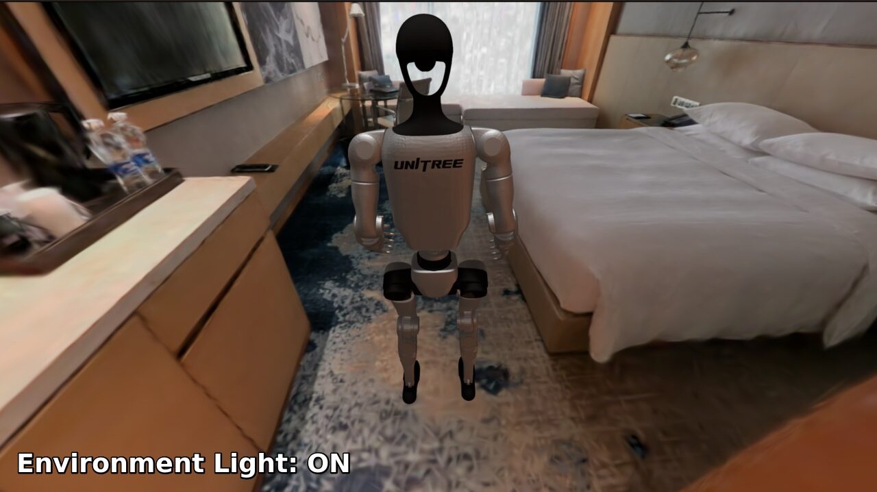
To integrate the robot into the scanned scene, its lighting must also harmonize with the background. 3DGS preserves the lighting appearance at scan time, while the newly added robot mesh needs its lighting computed separately. MotrixSim supports generating Image-Based Lighting (IBL) from the environment, providing diffuse and specular ambient light contributions for PBR meshes so that the robot’s shading, color tone, and highlights better match the surrounding scene. Here, IBL affects the lighting of mesh materials; the 3DGS scene retains its original appearance.
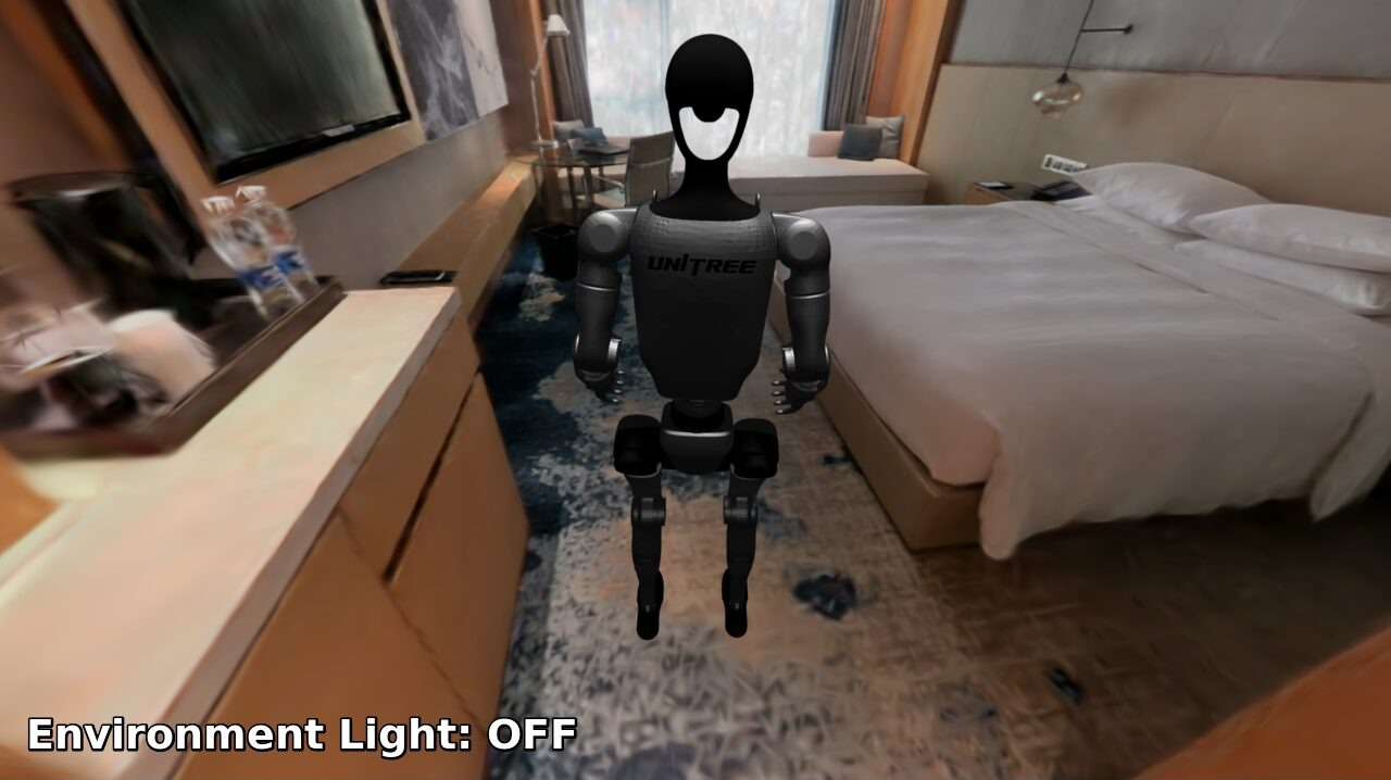
From Simulated Scenes to Synthetic Data
Once the visual scene is ready, MotrixGen can execute tasks in simulation and produce synthetic data. The Real2Sim2Real demonstration presents this process in a single frame: on the left, a single trajectory expands step by step into 20 simulated trajectories, showing MotrixGen executing tasks and generating data in the simulated scene; on the right, a task policy is trained with this synthetic data and deployed on a real robot for execution.
3.3BatchRender
Batched rendering for parallel environments MotrixSim’s renderer renders entire batches of multiple, parallel physics environments at once, producing images with shape (batch, tile_h, tile_w, Channel).
Dimension semantics batch is the number of parallel environments, aligned with the batch dimension of the physics data; tile_h and tile_w are the height and width of a single environment’s tile, i.e. that environment’s observation resolution; Channel is the number of channels — 3 for RGB and 4 for RGBA. Environment tiles are packed inside an atlas; slicing along dimension 0 extracts a single environment’s image, with no need for per-environment capture.
Output formats Cameras can output RGBA, Depth, SegmentationColor, and IdColor on demand: RGBA is the color image, Depth outputs depth only, SegmentationColor outputs segmentation coloring, and IdColor colors objects by id. All formats share the same batch layout and switch with the observation configuration; for depth-value conversion and the meaning of the segmentation mapping, see Visual Sensors.
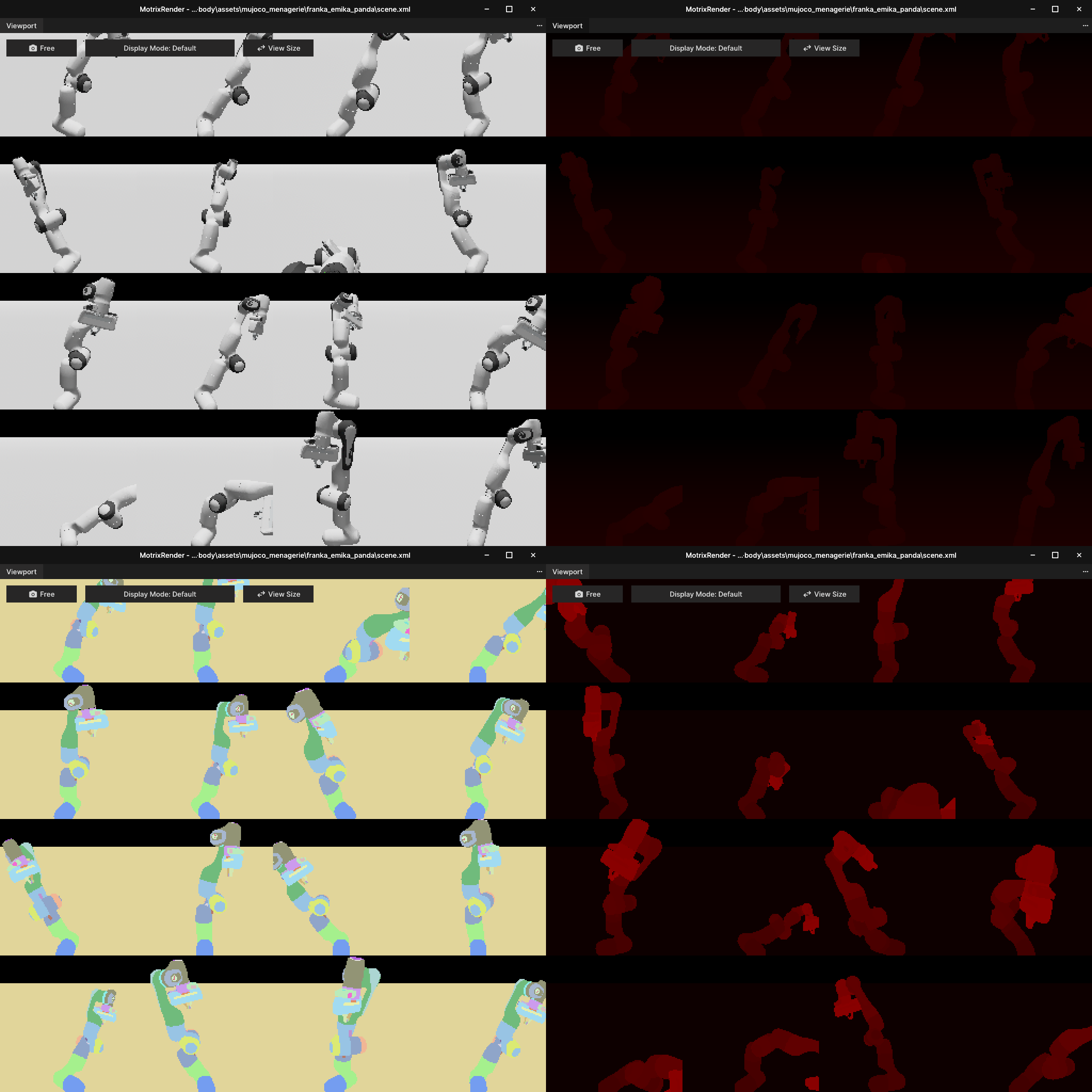
Images are tensors Rendered images can be consumed directly as tensors downstream; apart from the linearization of the atlas inside the GPU, there are no extra copies. The array shape is exactly (batch, tile_h, tile_w, Channel), with dimension 0 matching the batch dimension of the physics data, so it can be fed straight into the training loop as the policy network’s observation tensor.
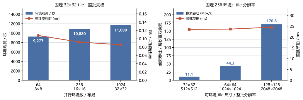
Throughput With a fixed 32×32 tile, scaling the full-batch layout from 8×8 to 32×32 grows the full-batch beat from 6.9 ms to 87.6 ms, yet per-environment observation throughput rises from about 9,277 to 11,690 observations/s and per-environment time drops from 0.108 ms to 0.086 ms — as the scale grows, the fixed cost of each synchronization is amortized, and throughput scales slightly better than linearly.
| Environments | Layout | Full-batch resolution | Full-batch beat | p95 | Observations/s | Per-environment time |
|---|---|---|---|---|---|---|
| 64 | 8×8 | 256×256 | 6.90 ms | 7.69 ms | 9,277 | 0.108 ms |
| 256 | 16×16 | 512×512 | 23.53 ms | 24.88 ms | 10,880 | 0.092 ms |
| 1024 | 32×32 | 1024×1024 | 87.60 ms | 93.74 ms | 11,690 | 0.086 ms |
Resolution With the environment count and layout fixed (256 environments, 16×16), raising the per-environment tile from 32×32 to 128×128 multiplies the full-batch pixel count 16×, yet a single synchronization only rises from 23.53 ms to 24.56 ms. Batch-rendering overhead is dominated by the fixed cost per synchronization rather than pixel fill, so increasing observation resolution costs almost no throughput.
| Tile per environment | Full-batch resolution | Full-batch beat | Observations/s | Pixel throughput |
|---|---|---|---|---|
| 32×32 | 512×512 | 23.53 ms | 10,880 | 11.1 Mpx/s |
| 64×64 | 1024×1024 | 23.68 ms | 10,813 | 44.3 Mpx/s |
| 128×128 | 2048×2048 | 24.56 ms | 10,424 | 170.8 Mpx/s |
4Sensors
4.1Sensor Overview
MotrixSim’s sensing capabilities can be grouped into four categories by observation source: proprioceptive state, contact and touch, environment geometry, and visual observations. They span the observation range from low-dimensional states to high-dimensional images, and can be provided to control, planning, and reinforcement learning modules through a unified interface.
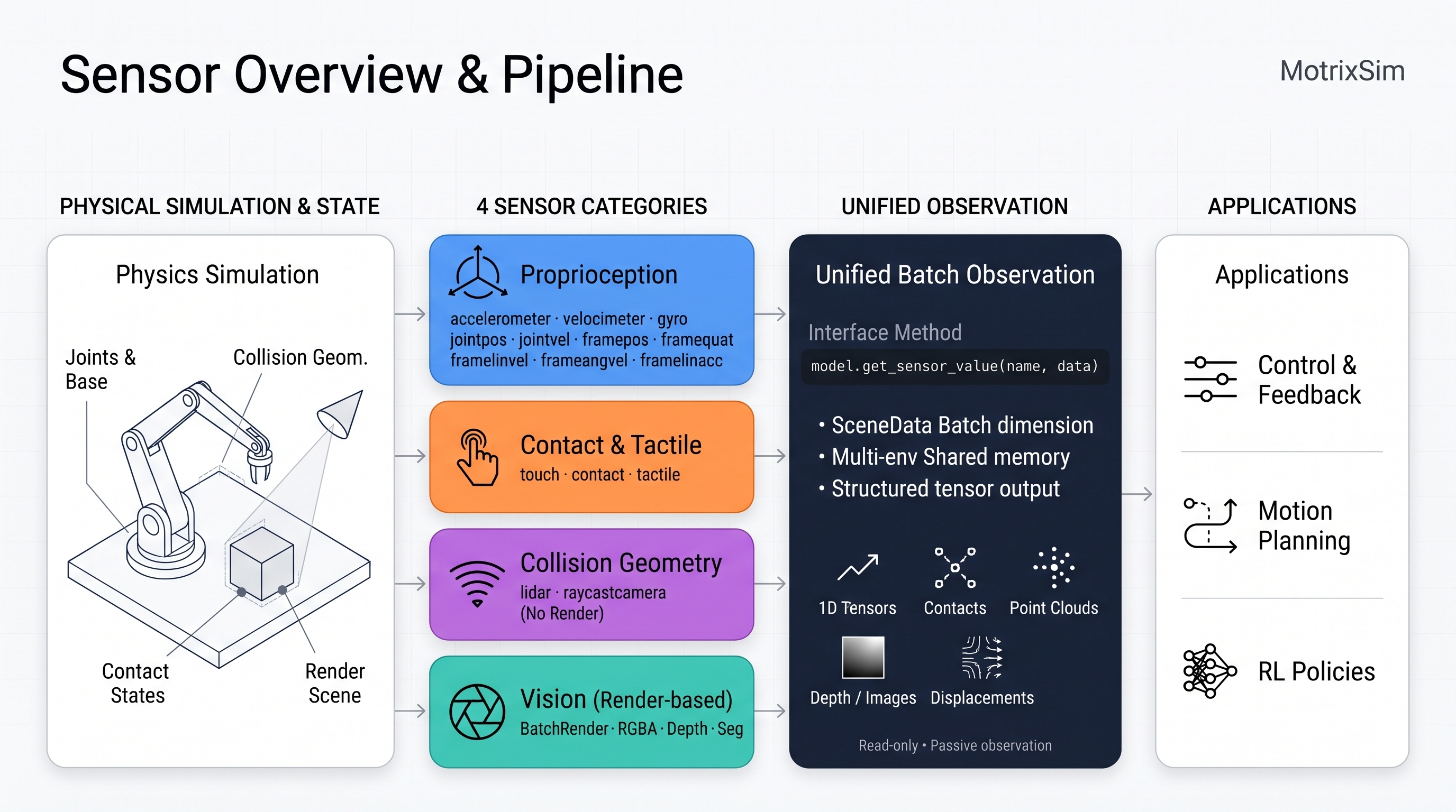
Proprioceptive State: Reading the Robot’s Own Motion
Proprioceptive state is the most commonly used low-dimensional input for controllers and policy networks. MotrixSim can read the robot’s own motion state from reference points (sites) and joints on the robot, including position, orientation, velocity, and acceleration, covering proprioceptive observation needs in feedback control, motion estimation, and reinforcement learning.
| Observation level | Data form | Typical uses |
|---|---|---|
| Local and joint states | Three-axis motion quantities, joint states | Feedback control, motion estimation, proprioceptive observations |
| Object and whole-body states | Pose, relative motion, center of mass and momentum | Task-space control, stability analysis, whole-body control |
Contact and Touch: Observing Whether and How Interaction Occurs
Contact observations convert local interactions from collision solving into signals usable by control and policies. They can either use a single normal-force scalar to quickly detect contact, or retain contact points and force details; touch simulation further describes the deformation of gel surfaces, suitable for fine manipulation.
| Observation level | Data form | Typical uses |
|---|---|---|
| Contact events and force sensing | Contact state, normal force, contact points and force attributes | Touchdown detection, grasp feedback, collision analysis |
| Soft contact and touch | Marker motion, 3D displacement fields, normal deformation | Fine grasping, visuotactile observations |
Environment Geometry: Directly Querying the Physics Collision Scene
LiDAR and RaycastCamera do not depend on the renderer; they directly perform ray queries against the geometry that participates in physical collision. They output distances, point clouds, or surface information, suitable for constructing environment observations in headless and massively parallel settings.
| Data form | Typical output | Typical uses |
|---|---|---|
| Multi-beam distance observations | Distances, world-frame point clouds, optionally acquisition time and surface normals | Obstacle avoidance, terrain perception, localization and mapping |
| Depth and surface observations | Depth, world-frame hit points, surface normals | Depth perception, terrain / height sampling |
Visual Observations: Generating Image Inputs from the Rendered Scene
Visual observations generate image inputs from the rendered scene that are commonly used by policy networks and vision algorithms. Beyond RGB color images, they can also output depth and segmentation or identification images colored by object id; they complement collision-geometry sensors — the former describes the rendering result, the latter the physics collision scene. For the uses of each output type, camera configuration, and the meaning of depth values, see visual sensors.
| Observation form | Output | Typical uses |
|---|---|---|
| RGB / RGBA | RGBA | Color perception, vision-based policies |
| RGB-D | RGBA + Depth | Depth perception, 3D scene understanding |
| Segmentation and object identification | SegmentationColor, IdColor | Instance and part discrimination, mask extraction, visualization |
4.2High-Performance LiDAR Simulation
LiDAR provides environment geometry observations for localization, mapping, and obstacle avoidance. MotrixSim performs distance queries against the scene’s collision geometry along scan directions, outputting distances and world-frame point clouds, and supports multiple sensors per scene as well as batched observations across many environments.
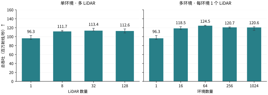
MotrixSim’s LiDAR simulation reaches a total throughput of up to about 124 million rays per second. On the CPU path of an AMD Ryzen 9 9950X with 32 threads, 64 parallel environments each carry a 1024×64 LiDAR, supporting batch generation of high-density point clouds.
4.3High-Precision Tactile Sensors
Fine manipulation depends on perceiving local contact: press depth, contact-patch shape, and subtle deformation of the gel surface are often hard to resolve visually, yet determine whether a manipulation succeeds. MotrixSim derives the contact region on the gel from rigid-body contact geometry, then obtains the 3D displacement field of the gel surface through a reduced-order contact solve, outputting the marker motion and normal-deformation observations commonly used by vision-based tactile sensors — all massively parallel with the physics simulation.
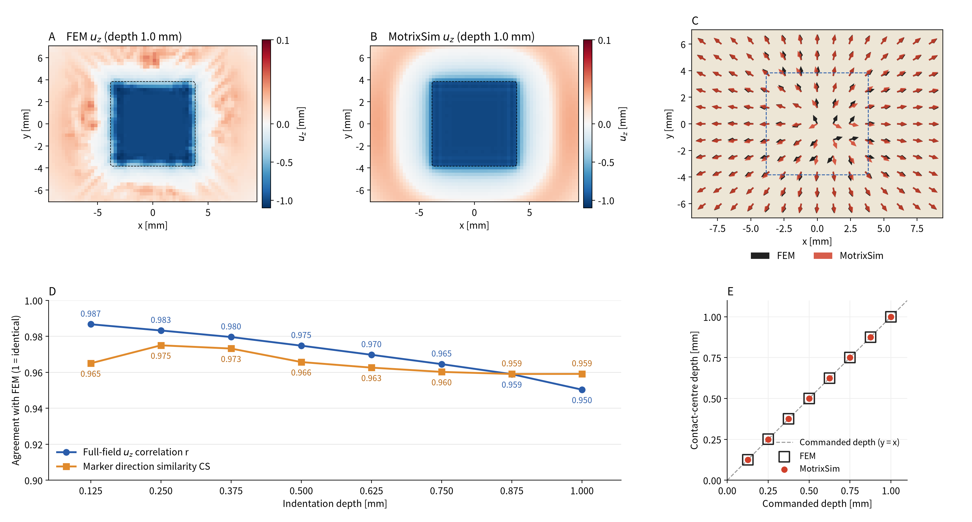
MotrixSim’s tactile output agrees closely with a nonlinear finite-element (FEM) reference solution. For a 7.5 mm cube press across 8 press depths from 0.125–1.0 mm, comparing MotrixSim’s raw (unsmoothed) tactile output with FEM, the full-field correlation coefficient of the normal displacement uz is 0.950–0.987, and the mean cosine similarity of marker in-plane displacement directions is 0.959–0.975; the press depth at the contact-region center deviates from FEM by no more than 1.04 µm, with a relative error of at most 0.70%.
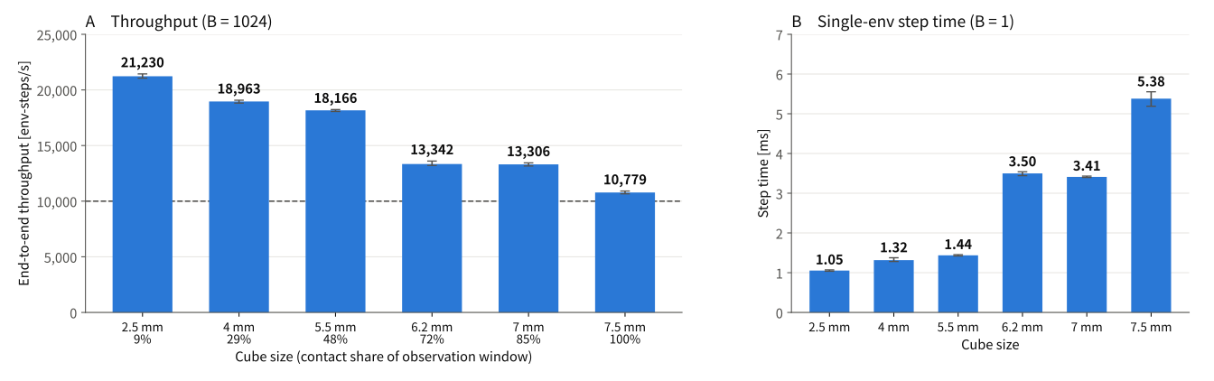
Tactile simulation can run massively in parallel together with the physics simulation. With 1024 parallel environments, MotrixSim’s tactile simulation achieves an end-to-end throughput of 10,800–21,200 env-steps/s (the summed number of environment steps advanced per second), with throughput decreasing as the contact area grows; even when the contact region fills the entire tactile observation window, throughput still exceeds 10,000 env-steps/s. The test platform is an NVIDIA GeForce RTX 5060 Ti with an Intel Core i5-14600KF; the tactile output is the 3D displacement field of the gel surface on a 64×48 grid, with physics and tactile step sizes of 1 ms.
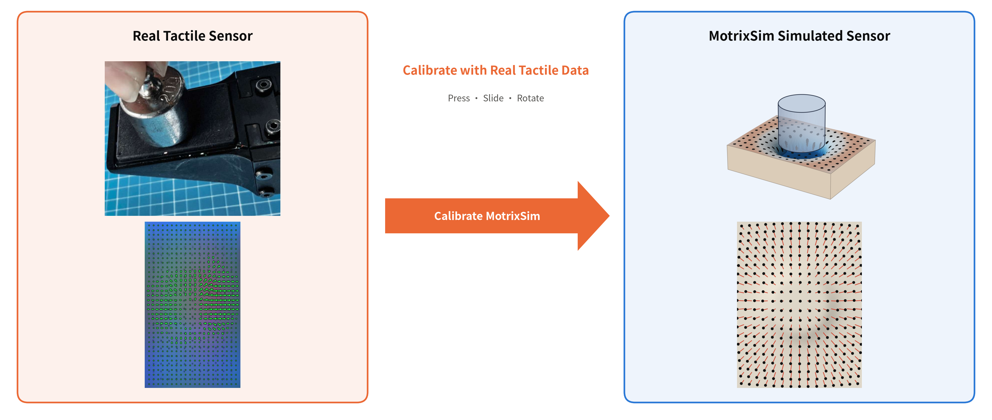
Calibrate MotrixSim with real tactile data to reproduce the response of a specific sensor in simulation. Tactile data from the real sensor are collected under known conditions such as pressing, sliding, and rotation, and used to calibrate MotrixSim’s simulation parameters so that the simulated sensor reproduces the tactile response of the same sensor, ready for large-scale training and deployment.
4.4Visual Sensors
MotrixSim provides color, depth, and geometry segmentation observations from the same simulated scene, supplying image inputs for visual perception, policy training, and synthetic data generation. Color images present the scene’s appearance, depth describes the spatial structure, and segmentation identifies which geometry each pixel belongs to, allowing appearance observations to be used together with part masks.
The figure below shows multiple outputs from the same camera and the same frame: the color image preserves materials and lighting, the depth map presents near-far relationships, and the two segmentation encodings target visualization and programmatic reading respectively. This information covers needs ranging from RGB perception and RGB-D scene understanding to part-level annotation. Segmentation is based on geometry (geom) identifiers; object or semantic class labels can be further mapped through the correspondence between geometries and objects/classes.
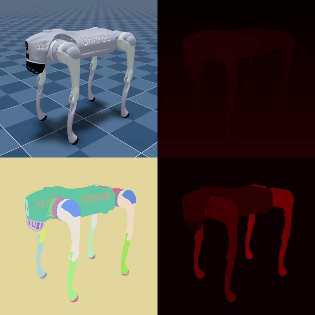
| Output | Content | Typical uses |
|---|---|---|
RGBA | Color image with alpha channel | Vision-based policies, perception, and synthetic data generation |
Depth | Depth along the camera optical axis (ViewZ) | RGB-D observations, 3D scene understanding |
SegmentationColor | Colored from a palette by geom id | Visual inspection, part discrimination |
IdColor | Encodes geom id as color | Programmatic id reading, mask extraction |
Visual observations and physical interaction share the same scene state. The physics solver updates the poses of robots and objects, and rendering uses these poses to generate images, so the motion process can be observed both through appearance and described through depth and geometry identifiers. For vision-based policies and interaction data generation, this links the image inputs to the scene that produces the motion and contact, rather than merely generating a set of standalone images.
The demo below shows the scene viewport together with camera outputs in the same frame, presenting depth and segmentation observations in a dynamic scene: the former presents the spatial structure from the camera’s viewpoint, and the latter distinguishes robot parts from environment geometries.
5Motion Planning and Control
5.1Motion Planning Library
MotrixSim ships with an efficient motion planning library that converts a “goal pose” into collision-free joint trajectories the robot can execute. It targets manipulator grasping, object transport, obstacle-avoiding motion in cluttered environments, and validating and executing planning results in simulation, connecting goal specification, path search, and physical interaction. For embodied-AI tasks, the planning library lets a robot go beyond “where to reach” to executable actions that specify “along which path and at what speed to get there”.
request = MotionPlanRequest(
    CartesianGoal(
        PointPositionGoal(position, POSITION_TOLERANCE),
        QuaternionOrientationGoal(orientation, ORIENTATION_TOLERANCE),
    ),
)
// With a single simple call, the planner returns an executable collision-free joint trajectory for the simulation to run.
trajectory = planner.plan(scene_data, request)
The following video shows the motion planning library applied to grasping and transport tasks
5.2Planning Benchmarks
Going further, we wanted to quantify MotrixSim’s motion planning capability on benchmarks. We evaluate MotrixSim’s planning with two public problem sets curated by Robometrics[2] under unified task inputs:
- MotionBenchMaker[3]: the problem sets used here include shelves, boxes, cage-like obstacles, and tabletop/under-table pick scenarios, probing the arm’s ability to reach targets in constrained spaces while avoiding obstacles.
- MπNets[4]: the problem sets used here cover grid shelving, drawer cabinets, and tabletop scenarios with varying start and goal configurations, probing the planner’s adaptability across diverse layouts and goal positions.
The evaluation exercises the full planning pipeline, from inverse kinematics and collision-free path search to trajectory time parameterization. A successful trajectory must satisfy an end-effector position error of at most 5 mm and an orientation error of at most 0.05 rad, and pass an independent collision check. The success rate reflects planning reliability, Plan Time measures the compute time to generate a trajectory, Position Error measures goal-position accuracy, and Motion Time denotes the duration of the planned trajectory.
MotrixSim achieved a 98.42% planning success rate on 2590 valid problems, with a median plan time of 34 ms on successful problems. The two problem sets comprise 2600 problems in total; the upstream marked 10 of them as infeasible goals and skipped them, and we follow that convention, computing the success rate over the remaining 2590 valid problems.
| Dataset | Valid Problems | Solved | Success Rate |
|---|---|---|---|
| MotionBenchMaker | 799 | 779 | 97.50% |
| MπNets | 1791 | 1770 | 98.83% |
| Total | 2590 | 2549 | 98.42% |
| Metric | Mean ± Std | Median | P75 | P98 |
|---|---|---|---|---|
| Plan Time (s) | 0.059 ± 0.136 | 0.034 | 0.062 | 0.322 |
| Position Error (mm) | 0.973 ± 1.11 | 0.501 | 1.50 | 4.22 |
| Motion Time (s) | 4.02 ± 4.86 | 2.91 | 4.14 | 20.43 |
The three metrics above cover successful problems only. Plan Time is the wall-clock time of a single planning call, excluding scene construction and independent result re-checking; Position Error is the end-effector position error at the trajectory's final point; Motion Time is the trajectory duration after time parameterization. Discrete collision checks are not a proof of continuous-path collision freedom.
6Developer Workflows
6.1Asset Import and Format Support
motrixsim.load_model(path) uniformly accepts MJCF, URDF, and USD, returning a SceneModel ready for simulation. The three formats can also be mixed within the same scene, for example placing an MJCF robot into a USD scene. Existing MuJoCo models and USD scene assets load and run as-is, with no format conversion in between.
Loading side by side with native engines
Two videos load the same asset side by side into MotrixSim and the corresponding native engine (MJCF into MuJoCo, USD into Isaac Sim), comparing physical behavior and scene rendering after loading.
USD support scope
MotrixSim reads USD assets through OpenUSD; .usd / .usda / .usdc / .usdz all load directly, and the expanded prims map to model elements such as rigid bodies, joints, geometry, and lights. Coverage is as follows; see the public USD support reference documentation for an item-by-item mapping:
- Fully supported: hierarchy and transforms, rigid bodies and joints (including mass properties), geometry and mesh collision, common lights.
- Partially supported: materials, scene properties, and drive parameters.
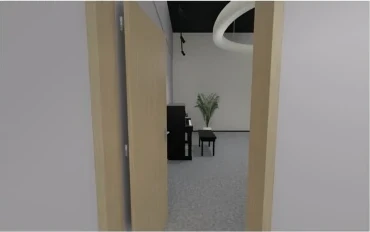
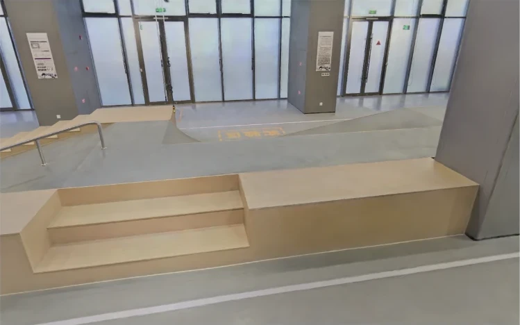
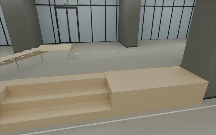
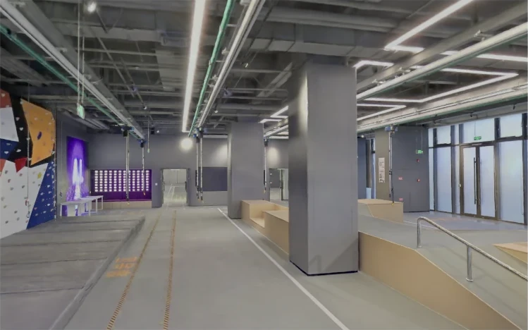
6.2Real2Sim: From Real Scenes to Interactive Simulation
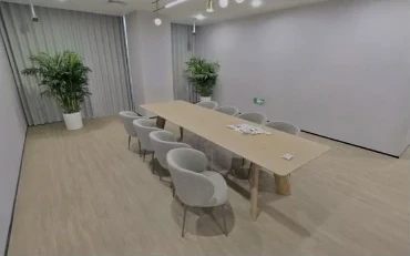
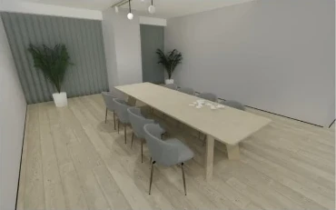
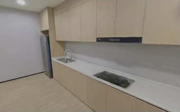
Turn real environments into interactive simulated scenes, so robot tasks unfold in familiar spaces. Real2Sim does more than reproduce scene appearance; it also organizes object layouts, structures, and kinematic relationships. By bringing the spatial layout and interactive objects of a real environment into MotrixSim, you can build the corresponding simulation environment for robot manipulation, task validation, and data collection.
Real scene
MotrixSim
Real scene
MotrixSim
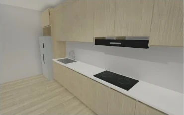
Real scene
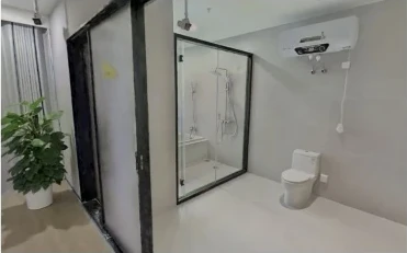
MotrixSim
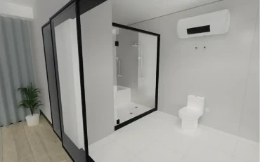
Real scene
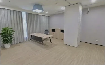
MotrixSim
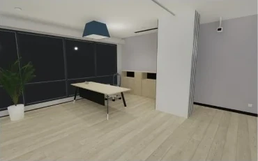
Real scene
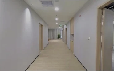
MotrixSim
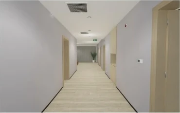
Real scene
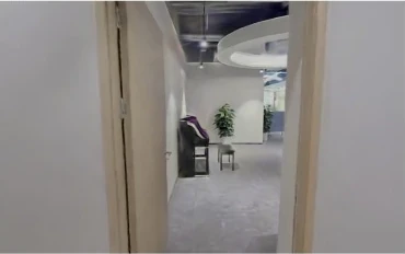
MotrixSim
Real scene
MotrixSim
Real scene
MotrixSim
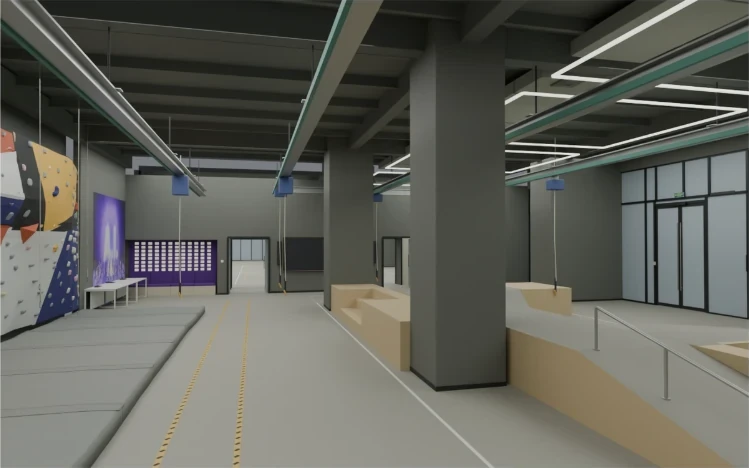
Real scene
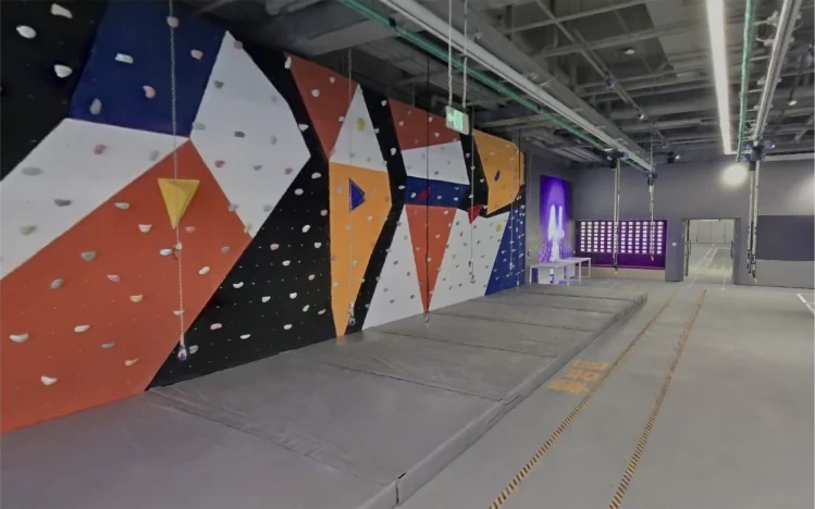
MotrixSim
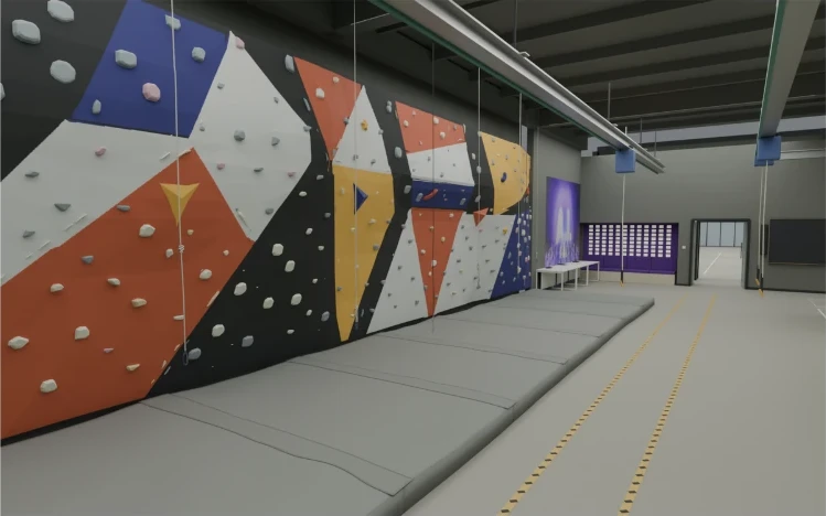
Real scene
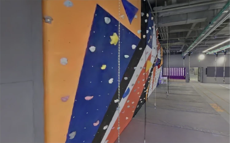
MotrixSim
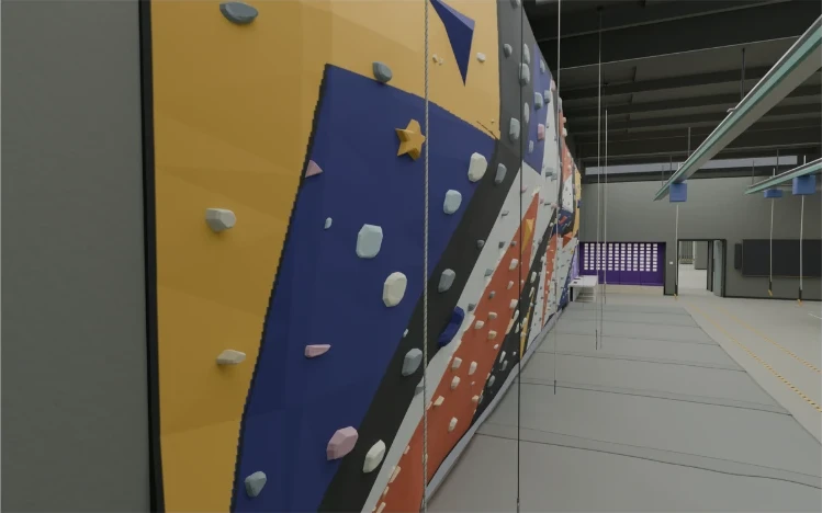
Real scene
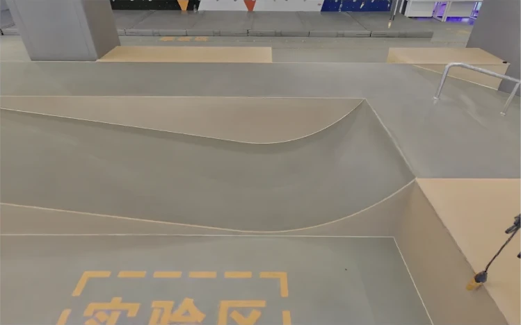
MotrixSim
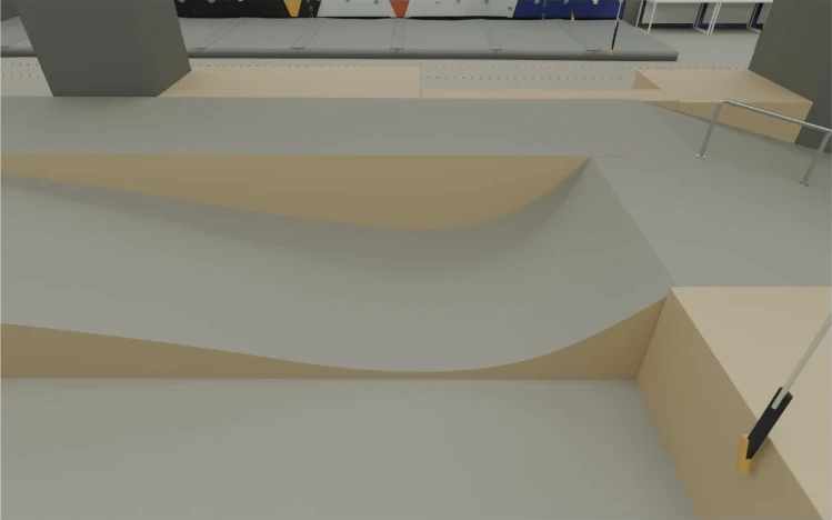
Real scene
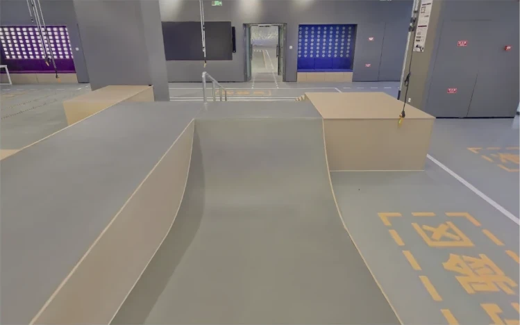
MotrixSim
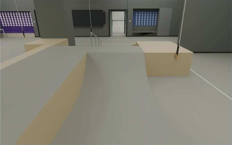
From scene reproduction toward operable objects. Objects such as cabinet doors and refrigerators are not just static appearances; they also include hinge structures that can open and close. The case below shows opening and closing motions in the simulated scene, extending environment reconstruction to object interaction and laying a scene foundation for subsequent robot manipulation.
Robot-scene interaction connects environment reproduction to task execution. The G1 case further shows a clip of a robot task simulated in MotrixSim.
6.3Forge Asset Tools
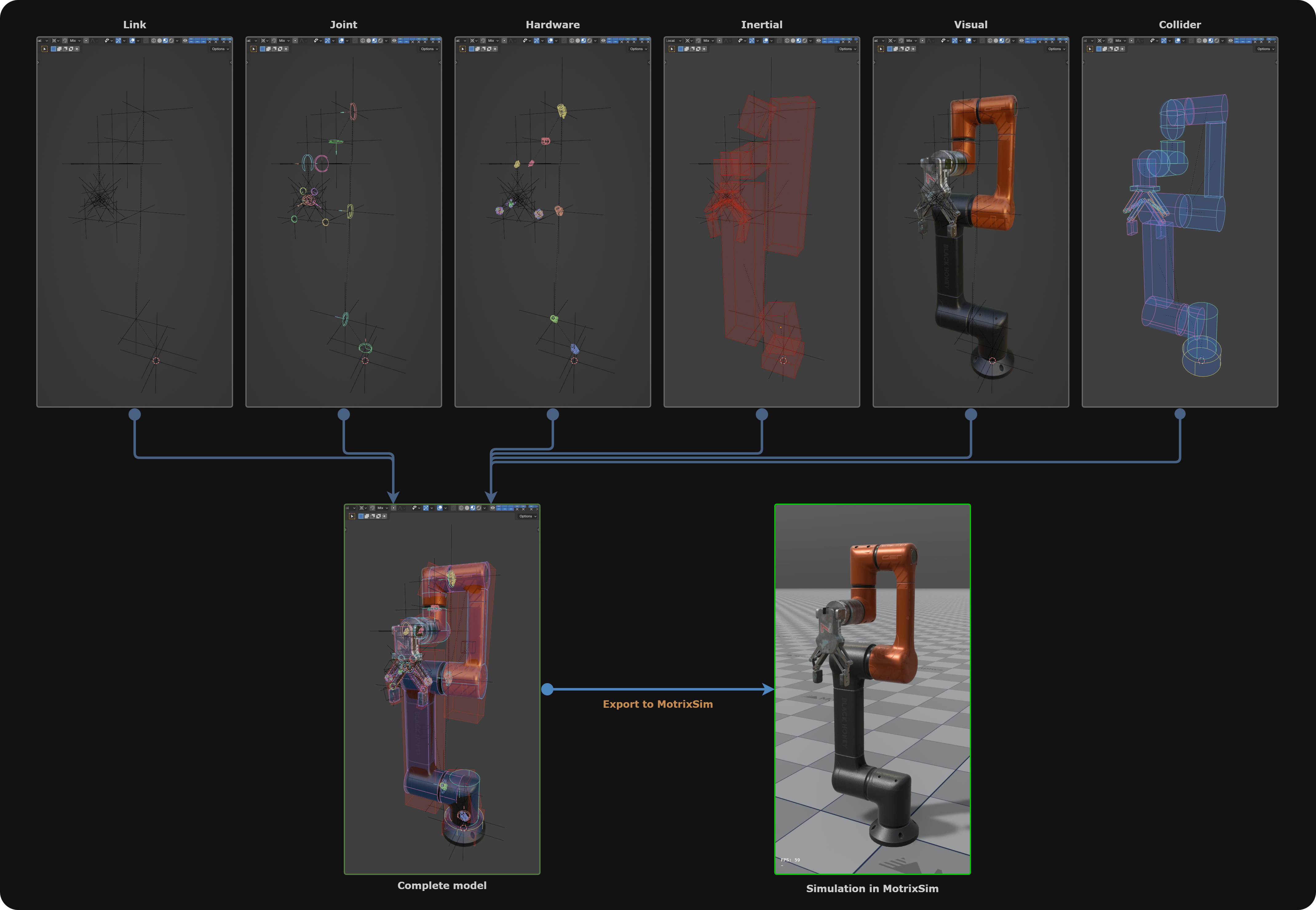
Forge is an efficient extension tool for creating, editing, and configuring XML scenes that precisely describe articulated multibody systems — kinematic structure, inertial properties, visual geometry, collision geometry, actuators, and sensors. It primarily addresses the lack of visual editing tools for MJCF and simplifies the creation, editing, and configuration of XML scene descriptions. Its core is the Forge plugin together with its companion MCP Server. The tool supports creating, editing, inspecting, and importing/exporting MJCF scene descriptions in Blender, and can also expose Forge capabilities to AI agents such as Codex and Claude Code via MCP.
Because MJCF has no visual editing tools, editing XML scenes under complex descriptions used to be disastrous. We therefore built the Forge plugin on top of the open-source Blender application to break down this barrier, making the creation/editing/configuration of XML scenes extremely easy.
Key Features
- Create MJCF model structures: create and organize model elements such as Link, Joint, Geometry, Collider, Site, Inertial, Actuator, Tendon, Sensor, Equality, Contact, Light, and Camera;
- Edit model definitions and properties: configure Global/General parameters, model types, geometries and materials, kinematics, hardware, Meta Elements, as well as parent-child relationships, root Link, instance Link, and transform properties;
- Interactive in-viewport editing: adjust MJCF properties of shapes, Links, Joints, Actuators, Tendons, Sensors, and more through the Forge panel, properties panel, and Gizmos, with live inspection of the scene structure;
- Import and export: import existing MJCF-standard .XML files and convert them into Forge-structured scenes, or export Forge-configured scene structures as MJCF-standard .XML files, and save the Blender project file;
- Mesh and collision handling: perform mesh checks and use CoACD to decompose complex meshes into convex hulls usable for collision detection;
- MCP automation: via MCP Bridge, let agents such as Claude Code and Codex query scenes, invoke Forge Operators, create or modify models, run imports/exports, and check multibody relationships.
Component Decomposition
Use Cases
6.4Editor and Scene Debugging
Scene debugging requires correlating control inputs, object motion, and runtime state so that an anomaly can be traced back to its cause. MotrixSim organizes the debugging workflow around Python task scripts and a standalone Editor, connecting task interaction, scene observation, and object inspection.
Python script debugging
Python debugging keeps task control and visualization in the same script. The developer loads models, writes control logic, and advances the simulation, observes the scene through a RenderApp, and builds a task control panel with a custom UI. Buttons, toggles, and selection widgets can be wired to script logic for target switching, task start/stop, reset, and display settings; the control panel can further be combined with a 3D viewport, status logs, and image panels, arranged to fit the debugging need.
In a robotic-arm pick-and-place example, task, state, configuration, and logs are organized in collapsible groups, shown side by side with a robot overview and a gripper close-up. After selecting a target and starting the task, the developer can inspect the motion path in the overview, examine the approach and grasping phases in the close-up, and use stage logs and curve changes to pinpoint when an anomaly occurred. After adjusting control logic or scene configuration, re-running and comparing results verifies the effect of the change.
Standalone Editor scene debugging
The standalone Editor targets scene inspection after model integration, linking the scene tree, viewport selection, and property panels so that object hierarchy, spatial placement, and physical state are connected. When diagnosing a gripper making premature contact, you can overlay collision shapes against the visible model with helper visualizations; when diagnosing anomalous motion, you can combine joint positions, reference frames, plus actuator, sensor, and contact information to progressively narrow down the problem.
The viewport and tool panels support docking, splitting, and tabbed combinations, making it easy to view overall motion, local geometry, and state information side by side. Unified toolbar icons help users recognize common functions across panels; the log panel supports reading long text, search, filtering, and auto-following, for tracing run records around the moment an anomaly appears.
In the future, the standalone Editor will also support built-in Python logic, so that script-driven task interaction and object inspection can be combined in the same workspace.
Python scripts and the standalone Editor emphasize task-logic iteration and scene-object inspection respectively, together supporting the debugging process from running and observing to localizing and verifying.
7Conclusion
Across the history of intelligent technology, every leap in capability has been driven by a collapse in the cost of acquiring some key resource. The internet made text and images accumulate at near-zero cost, giving rise to today’s language models; experience in the physical world is the opposite — expensive, slow, dangerous, and nearly impossible to reproduce. For physical AI to form a scalable learning loop, physical experience must first become as copyable, composable, and mass-producible as data. This is simulation’s new position in the era of physical AI: no longer merely a verification tool at the end of the development pipeline, but a production system for physical experience.
This capability deserves to be built as infrastructure precisely because its foundation is shared across industries. A vehicle, an excavator, a production line, and a robot arm all face the same problem: making decisions from observation in an uncertain environment and bearing the physical consequences of their actions. Every advance on this common problem — more trustworthy contact, larger-scale parallelism, more complete multimodal feedback — simultaneously lowers the barrier for every industry to acquire physical experience. For the first time, the learning resources of physical AI can circulate and be reused across industries.
We are clear that this path is still in its early stages. MotrixSim will keep investing in trustworthy physics, computation at scale, and multimodal feedback, and will keep updating this report as application scenarios deepen. Our goal remains unchanged: to make physical interaction a scalable, generative learning resource, so that more exploration happens first in the virtual world.
8References
- Karlsruhe Institute of Technology. Tire bench-test dataset (TYDEX format), 32 files, 1015 operating points. doi:10.35097/p0rr2jc5wmf0drf8
- fishbotics/robometrics: robot motion evaluation framework, revision 81e3d1d6. github.com/fishbotics/robometrics
- C. Chamzas, C. Quintero-Peña, Z. Kingston, A. Orthey, D. Rakita, M. Gleicher, M. Toussaint, and L. E. Kavraki. MotionBenchMaker: A tool to generate and benchmark motion planning datasets. IEEE Robotics and Automation Letters, 2022. doi:10.1109/LRA.2021.3133603
- A. Fishman, A. Murali, C. Eppner, B. Peele, B. Boots, and D. Fox. Motion Policy Networks. CoRL, 2022. arXiv:2210.12209
9Appendix
Data Sources and Test Conditions (Vehicle Dynamics)
- Spring and damper curves use synthetic example data to demonstrate nonlinear component configuration.
- Single-environment performance was measured with MotrixSim 0.10.1, an AMD Ryzen 7 9700X, one worker, f32 precision, and a 5 ms time step. Five runs followed 400 warm-up steps; timing covers physics stepping only. Parallel throughput was measured on an asynchronous sampling node with 96 CPUs and one RTX 3090. Results use an independently calibrated vehicle; raw records are not included in the public repository.
Magic Formula Equations and Symbol Definitions
The Magic Formula maps slip to nonlinear tire forces. The following gives its basic form for the force magnitude under pure longitudinal or pure lateral slip, consistent with the characteristic curves in the main text; longitudinal and lateral directions use their own fitted parameters:
| Symbol | Definition and role |
|---|---|
| i | Direction subscript: x is the tire longitudinal direction, y is the lateral direction; the two directions are fitted separately. |
| s | Input of the constitutive curve: the absolute slip ratio |κ| longitudinally, the absolute slip angle |α| laterally. |
| κ | Longitudinal slip ratio, dimensionless, describing the relative difference between the tire’s circumferential speed and its forward travel speed; zero for pure rolling. Percentages in the figures are κ × 100%. |
| α | Slip angle, the angle between the tire heading and the direction of the wheel-center velocity relative to the road; radians (rad) in the equations, degrees (deg) on the curve axes. |
| yᵢ(s) | Ratio of the tire force magnitude in direction i to the normal load, i.e. a dimensionless force coefficient; not the y coordinate in the geometry figure. |
| Bᵢ | Stiffness factor controlling the initial growth in the small-slip region; Bᵢs is dimensionless. Longitudinal Bₓ is dimensionless, lateral Bᵧ is expressed in rad⁻¹. |
| Cᵢ | Shape factor, dimensionless, controlling the overall curve shape. |
| Dᵢ | Peak factor, dimensionless, setting the peak scale of the force coefficient; the corresponding force scale is Fz · Dᵢ. |
| Eᵢ | Curvature factor, dimensionless, adjusting the curvature near the peak and the post-peak behavior. |
| Fx、Fy | Longitudinal and lateral ground forces on the tire, in N; absolute values denote magnitudes, with actual directions determined by slip and sign conventions. |
| Fz | Normal support force from the ground on the tire, in N, non-negative during contact; obtained from the normal contact solve, not from the MF tangential formulas above. |
Here sin is the sine function, arctan is the arctangent, and vertical bars denote absolute value. The slope of the force-coefficient curve at small slip is determined jointly by BᵢCᵢDᵢ; Bᵢ and Dᵢ may also vary with normal load to express load sensitivity.
In the geometry figure, R is the tire’s effective rolling radius (m), ω is the wheel’s spin rate (rad/s), and Rω is the circumferential speed (m/s); V is the wheel-center velocity relative to the road, with Vx and Vy its longitudinal and lateral tire-axis components (m/s). Wheel speed and translational velocity determine slip, normal contact determines load, and the tire’s tangential forces enter the full-vehicle dynamics solve, linking tire response to suspension and body motion.